GWAS Power Calculation

Haky Im

2021-01-24

Categories: vignette

Overview

We want to calculate the power to detect an association a genetic marker and a quantitative phenotype.

Write functions to simulate genotype and phenotype under an additive genetic model.
Simulate genotype and phenotype using the simulator under the null and alternative.
Select the relevant statistic and perform the hypothesis test.
Calculate the power of the test.

As a concrete example, we pre-specify the model for continuous trait \(Y\) and genotype \(X\) as

\[Y = \beta X + \epsilon, ~~~~ \text{with } \epsilon \sim N(0, \sigma_\epsilon^2)\]

where we assume

genotype of the locus follows Hardy-Weinberg equilibrium with a pre-specified minor allele frequency.
trait is normalized to variance 1 and the proportion of variation explained by the SNP is \(r^2\).

The goal is to calculate the power with the significance level (\(\alpha\)), effect size (in the form of \(r^2\)), and sample size (num_individuals).

Note that the proportion of variation explained, minor allele frequency, effect size (\(\beta\)) are related under the model above and you will be/have already been asked to work it out in assignment.

Phenotype-genotype simulator

To simulate genotype, we assume the locus is bialleilic and each individual is diploid. So that \(X \sim \text{Binomial}(2, f)\) with \(f\) as minor allele frequency (here we encode minor allele as 1 and major allele as 0).

Given genotype, to simulate phenotype, we need to know \(\beta\) and \(\sigma_\epsilon^2\). So, we first calculate the effect size and the variance of the noise term from the proportion of variation explained, variance of trait, and minor allele frequency of the SNP.

simulate_genotype = function(maf, num_individuals, num_replicates) {
  # maf: minor allele frequency
  # num_individuals: the number of individuals in each replicates
  # num_replicates: the number of replicates
  # it returns a matrix with num_individuals rows and num_replicates columns
  genotype = matrix( 
    rbinom(num_individuals * num_replicates, 2, maf), 
    nrow = num_individuals, 
    ncol = num_replicates 
  )
  return(genotype)
}
simulate_phenotype = function(genotype, beta, sig2epsi) {
  # genotype: each column is one replicate 
  # beta: effect size of the linear model
  # sig2epsi: the variance of the noise term
  num_individuals = nrow(genotype)
  num_replicates = ncol(genotype)
  epsilon = matrix( 
    rnorm(num_individuals * num_replicates, mean = 0, sd = sqrt(sig2epsi)), 
    nrow = num_individuals, 
    ncol = num_replicates 
  )
  phenotype = genotype * beta + epsilon
  return(phenotype)
}
get_beta_and_sig2epsi = function(r2, sig2Y, maf) {
  # r2: proportion of variation explained by SNP
  # sig2Y: variance of trait
  # maf: minor allele frequency of SNP
  # it returns a list of beta and variance of noise term
  
  ## effect size is calculated from r2 = beta^2 *2*maf*(1-maf)
  beta = sqrt( r2 * sig2Y / (2 * maf * (1 - maf)) )
  sig2epsi = sig2Y * (1 - r2)
  return(list(beta = beta, sig2epsi = sig2epsi))
}
linear_model_simulator = function(num_replicates, num_individuals, maf, r2, sig2Y) {
  # simulate genotype
  X = simulate_genotype(maf, num_individuals, num_replicates)
  # calculate model parameters
  params = get_beta_and_sig2epsi(r2, sig2Y, maf)
  # simulate phenotype given genotype and model parameters
  Y = simulate_phenotype(X, params$beta, params$sig2epsi)
  return(list(Y = Y, X = X))
}

Simulate 10,000 Y vectors under null and alternative scenarios

Here we simulate 1000 individuals per replicate and 10000 replicates in total. With parameters: * Minor allele frequency is 0.3. * Proportion of variance explained is 0.01 * Variance of trait is 1.

# specify paramters
nindiv = 1000
nreplicate = 10000
maf = 0.30
r2 = 0.01
sig2Y = 1

# run simulator 
## under the alternative
data_alt = linear_model_simulator(nreplicate, nindiv, maf, r2, sig2Y)
dim(data_alt$Y)

## [1]  1000 10000

dim(data_alt$X)

## [1]  1000 10000

## under the null
data_null = linear_model_simulator(nreplicate, nindiv, maf, 0, sig2Y)  
dim(data_null$Y)

## [1]  1000 10000

dim(data_null$X)

## [1]  1000 10000

define functions to run associations and obtain the z-scores

runassoc = function(X,Y)
{
  pvec = rep(NA,ncol(X))
  bvec = rep(NA,ncol(X))
  for(ss in 1:ncol(X))
  {
    fit = fastlm(X[,ss], Y[,ss])
    pvec[ss] = fit$pval  
    bvec[ss] = fit$betahat
  }
  list(pvec=pvec, bvec=bvec)
}

p2z = function(b,p)
{
  ## calculate zscore from p-value and sign of effect size
  sign(b) * abs(qnorm(p/2))
}

calcz = function(X,Y)
{
  tempo = runassoc(X,Y)
  p2z(tempo$bvec,tempo$pvec)
}

Load some packages

library(tidyverse)

## ── Attaching packages ─────────────────────────────────────── tidyverse 1.3.0 ──

## ✓ ggplot2 3.3.3     ✓ purrr   0.3.4
## ✓ tibble  3.0.5     ✓ dplyr   1.0.3
## ✓ tidyr   1.1.2     ✓ stringr 1.4.0
## ✓ readr   1.4.0     ✓ forcats 0.5.0

## ── Conflicts ────────────────────────────────────────── tidyverse_conflicts() ──
## x dplyr::filter() masks stats::filter()
## x dplyr::lag()    masks stats::lag()

fastlm = function(xx,yy)
{
  ## compute betahat (regression coef) and pvalue with Ftest
  ## for now it does not take covariates

  df1 = 2
  df0 = 1
  ind = !is.na(xx) & !is.na(yy)
  xx = xx[ind]
  yy = yy[ind]
  n = sum(ind)
  xbar = mean(xx)
  ybar = mean(yy)
  xx = xx - xbar
  yy = yy - ybar

  SXX = sum( xx^2 )
  SYY = sum( yy^2 )
  SXY = sum( xx * yy )

  betahat = SXY / SXX

  RSS1 = sum( ( yy - xx * betahat )^2 )
  RSS0 = SYY

  fstat = ( ( RSS0 - RSS1 ) / ( df1 - df0 ) )  / ( RSS1 / ( n - df1 ) )
  pval = 1 - pf(fstat, df1 = ( df1 - df0 ), df2 = ( n - df1 ))
  res = list(betahat = betahat, pval = pval)

  return(res)
}

Now we can calculate test statistics under the null and alternative scenarios.

Zalt = calcz(data_alt$X, data_alt$Y)
Znull = calcz(data_null$X, data_null$Y)
## create a data frame to use ggplot
pp = tibble(Y = c(Zalt,Znull), type=c(rep("alt",length(Zalt)),rep("null",length(Znull))) ) %>% ggplot(aes(Y,fill=type)) + geom_density(color=NA,alpha=0.6) + theme_bw(base_size = 15)
pp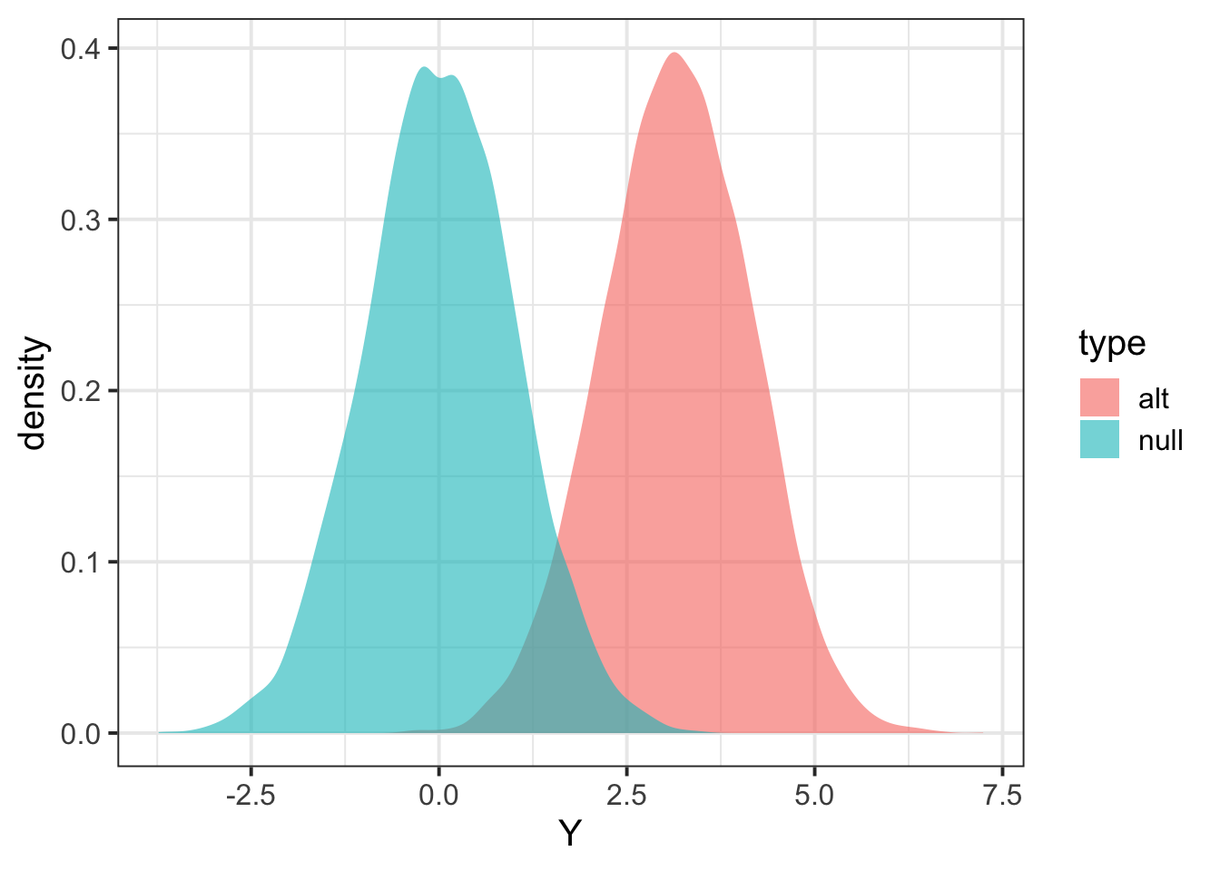

Calculate power

## define significance level (=type I error we are willing to accept)

alpha = 0.01

## find threshold for rejection; we want P(Znull > alpha/2) two-sided

threshold = quantile(Znull, 1 - alpha/2)
print(threshold,2)

## 99.5% 
##   2.6

## add threshold to the Zscores figure
pp + geom_vline(xintercept=threshold,col='dark green',size=1.5)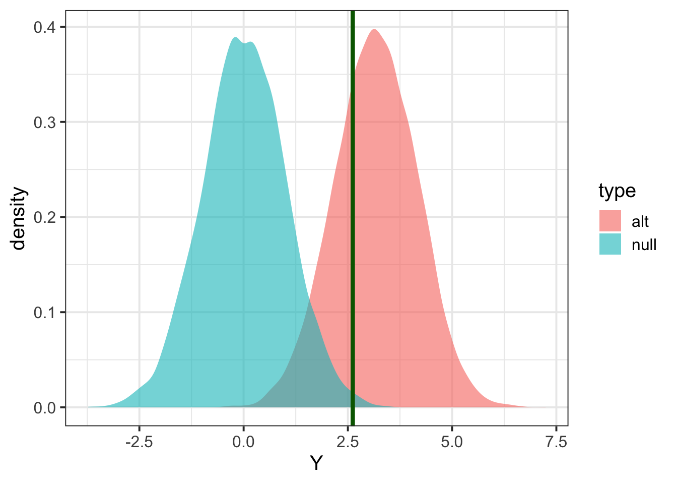

## calculate proportion of Zalt above threshold

power = mean(Zalt > threshold)
print(power)

## [1] 0.7106

## to be more precise, we should be calculating the proportion of null replicates that are either above or 
mean(Zalt > threshold | Zalt < -threshold)

## [1] 0.7106

## not much different since the probability of Zalt being negative is almost 0

check with pwr.r.test function

## install.packages("pwr")
if (!("pwr" %in% installed.packages()[, 1])) {
  install.packages("pwr")
}
pwr::pwr.r.test(n = nindiv, r= sqrt(r2), sig.level = alpha)

## 
##      approximate correlation power calculation (arctangh transformation) 
## 
##               n = 1000
##               r = 0.1
##       sig.level = 0.01
##           power = 0.7234392
##     alternative = two.sided