L4-power

Workflow overview

In this vignette, we’d like to:

1. Write a simulator to simulate genotype and phenotype under some pre-specified model.
2. Simulate genotype and phenotype using the simulator under the null and alternative.
3. Perform certain hypothesis test.
4. Calculate the power of the test.

As a concrete example, we pre-specify the model for continuous trait \(Y\) and genotype \(X\) as

\[Y = \beta X + \epsilon, \epsilon ~ N(0, \sigma_\epsilon^2)\]

where we assume

• genotype of the locus follows Hardy-Weinberg equilibrium with a pre-specified minor allele frequency.
• trait is normalized to variance 1 and the proportion of variation explained by the SNP is \(r^2\).

Note that the proportion of variation explained, minor allele frequency, effect size (\(\beta\)) are related under the model above and you will be/have already been asked to work it out in assignment.

Phenotype-genotype simulator

To simulate genotype, we assume the locus is bialleilic and each individual is diploid. So that \(X \sim Binomial(2, f)\) with \(f\) as minor allele frequency (here we encode minor allele as 1 and major allele as 0).

Given genotype, to simulate phenotype, we need to know \(\beta\) and \(\sigma_\epsilon^2\). So, we first calculate the effect size and the variance of the noise term from the proportion of variation explained, variance of trait, and minor allele frequency of the SNP.

simulate_genotype = function(maf, num_individuals, num_replicates) {
  # maf: minor allele frequency
  # num_individuals: the number of individuals in each replicates
  # num_replicates: the number of replicates
  # it returns a matrix with num_individuals rows and num_replicates columns
  genotype = matrix( 
    rbinom(num_individuals * num_replicates, 2, maf), 
    nrow = num_individuals, 
    ncol = num_replicates 
  )
  return(genotype)
}
simulate_phenotype = function(genotype, beta, sig2epsi) {
  # genotype: each column is one replicate 
  # beta: effect size of the linear model
  # sig2epsi: the variance of the noise term
  num_individuals = nrow(genotype)
  num_replicates = ncol(genotype)
  epsilon = matrix( 
    rnorm(num_individuals * num_replicates, mean = 0, sd = sqrt(sig2epsi)), 
    nrow = num_individuals, 
    ncol = num_replicates 
  )
  phenotype = genotype * beta + epsilon
  return(phenotype)
}
get_beta_and_sig2epsi = function(r2, sig2Y, maf) {
  # r2: proportion of variation explained by SNP
  # sig2Y: variance of trait
  # maf: minor allele frequency of SNP
  # it returns a list of beta and variance of noise term
  
  ## effect size is calculated as r2 = beta^2 *2*maf*(1-maf)
  beta = sqrt( r2 * sig2Y / (2 * maf * (1 - maf)) )
  sig2epsi = sig2Y * (1 - r2)
  return(list(beta = beta, sig2epsi = sig2epsi))
}
linear_model_simulator = function(num_replicates, num_individuals, maf, r2, sig2Y) {
  # simulate genotype
  X = simulate_genotype(maf, num_individuals, num_replicates)
  # calculate model parameters
  params = get_beta_and_sig2epsi(r2, sig2Y, maf)
  # simulate phenotype given genotype and model parameters
  Y = simulate_phenotype(X, params$beta, params$sig2epsi)
  return(list(Y = Y, X = X))
}

Run the simulator under the null and alternative

Here we simulate 1000 individuals per replicate and 10000 replicates in total. With parameters:

• Minor allele frequency is 0.3.
• Proportion of variance explained is 0.01.
• Variance of trait is 1.

# specify paramters
nindiv = 1000
nreplicate = 10000
maf = 0.30
r2 = 0.01
sig2Y = 1
# run simulator 
## under the alternative
data_alt = linear_model_simulator(nreplicate, nindiv, maf, r2, sig2Y)
## under the null
data_null = linear_model_simulator(nreplicate, nindiv, maf, 0, sig2Y)  

Perform hypothesis test

The following chunk of R code implement hypothesis test procedure based on linear regression. Essentially, the R function calcz takes genotype X and Y and returns test statistic z-score.

runassoc = function(X,Y)
{
  pvec = rep(NA,ncol(X))
  bvec = rep(NA,ncol(X))
  for(ss in 1:ncol(X))
  {
    fit = fastlm(X[,ss], Y[,ss])
    pvec[ss] = fit$pval  
    bvec[ss] = fit$betahat
  }
  list(pvec=pvec, bvec=bvec)
}
p2z = function(b,p)
{
  ## calculate zscore from p-value and sign of effect size
  sign(b) * abs(qnorm(p/2))
}
calcz = function(X,Y)
{
  tempo = runassoc(X,Y)
  p2z(tempo$bvec,tempo$pvec)
}

Now that we can calculate test statistics under the null and alternative.

Zalt = calcz(data_alt$X, data_alt$Y)
Znull = calcz(data_null$X, data_null$Y)
tibble(Y = c(Zalt,Znull), type=c(rep("alt",length(Zalt)),rep("null",length(Znull))) ) %>% ggplot(aes(Y,fill=type)) + geom_density(color=NA,alpha=0.6) + theme_bw(base_size = 15)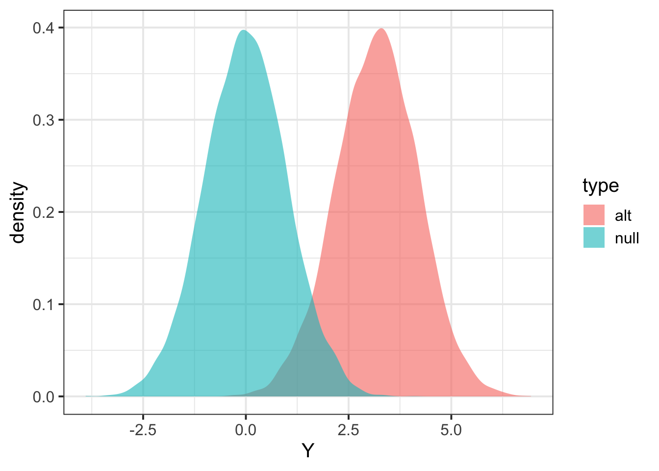

Calculate power

## define significance level
alpha = 0.01
## find threshold for rejection; we want P(Znull > alpha/2) two-sided
threshold = quantile(Znull, 1 - alpha/2)
## calculate proportion of Zalt above threshold
mean(Zalt > threshold)

## [1] 0.7516

check with pwr.r.test function

## install.packages("pwr")
 library(pwr)
pwr.r.test(n = nindiv, r= sqrt(r2), sig.level = alpha)

## 
##      approximate correlation power calculation (arctangh transformation) 
## 
##               n = 1000
##               r = 0.1
##       sig.level = 0.01
##           power = 0.7234392
##     alternative = two.sided