Created by Max Winston; modified by Charles Washington III, Ankeeta Shah, and Yanyu Liang
This class is designed to introduce a variety of concepts, methods, and tools utilized in statistical genetics. The majority of tools used to employ these methods and concepts require basic knowledge of computing languages, specifically Unix and R. In today’s lab, we will cover the basic syntax of these languages and some basic commands necessary for operating statistical genetics programs. By the end of this lab, you should understand how to perform the following:
- Navigate in R and Unix
- Download and install software packages in Unix
- Write looped bash commands to run in Unix
- Manipulate large text files in Unix
- Import data files into R
- Manipulate and visualize files in R
Commonly used commands in Unix
List of Basic Commands
| Command | Description |
|---|---|
| pwd | Print working directory (tells you where you are) |
| cd | Change directory |
| mkdir | Make directory |
| ls | List information about files |
| mv | Moves or renames files or directories |
| rm | Deletes files (can remove directories with -rf) |
| cp | Copy a file to a new location (can copy directories with -r) |
| scp | Secure copy a file (for transferring files between a remote server and local system) |
| cat | Concatenate and print the content of files to screen |
| sed | Stream editor (for searching, finding, and replacing text) |
| “pipe” | Uses the output of one command as the input for another |
| > | Writes output into file (must enter file name after, will overwrite) |
| >> | Writes output into file (must enter file name, will append, not overwrite) |
| curl | Transfer a URL (downloads something from the Internet) |
| wget | Transfer a URL (downloads something from the Internet) |
| tar | Creates tape archives and adds or extracts files |
| ssh | Remote log-in command (Secure Shell client) |
| emacs | Opens emacs text editor |
| vim | Opens vim text editor |
| nano | Opens nano text editor |
| man | Access manual for any command (exit = q) |
| top | Observe computer’s tasks |
| sort | Sorts a file (extensive options to direct this command) |
| head | Look at the first ten lines of file (useful for large files) |
| tail | Look at the last ten lines of file (useful for large files) |
| ./ | Existing directory (not a command) |
| ../ | Directory contaiing existing directory (not a command) |
| grep | Prints lines matching a pattern (helpful for manipulating large files) |
| SLURM specifics | Description |
|---|---|
| sbatch | Submits a job to the server |
| sinterative | Submits an interactive job to the server (Our labs will use it a lot) |
| squeue | Status of a job you’ve submitted to the server |
Logging in and moving files
For the remainder of the document, please notice that steps requiring actions will generally be in bold. For example, Open Terminal if you are on a Mac.
Each of you should have been assigned a username on the server. You will use a Secure Shell client to log in to your home directory on the server. You can do this by:
ssh <username>@midway2.rcc.uchicago.eduNote that you will be prompted to enter your password. One somewhat counter-intuitive facet of password entry in Unix is that there is no indiciation on-screen of characters being typed in. This is an intentional security feature, in order to prevent onlookers from inferring the length of your password. Type in your password when prompted. The midway2 server has recently implemented two-factor authentication, so you will next be prompted to log in with DUO, enter a passcode, or receive a call. After you do one of these three things, you should be on the server.
Using the commands listed above, do the following in your home directory:
- 1) Make your own directory.
- 2) Make a second directory.
- 3) Look where your directories live.
- 4) Move one of your directories into the other.
- 5) Change directory to your new directory.
- 6) Look inside your new directory.
- 7) Move to the original directory.
- 8) Read more about the rm command.
- 9) Delete both directories you’ve made.
- 10) Create a directory called for this lab session and move into it.
mkdir your_directory/         ##Step 1
mkdir dir_2/                  ##Step 2
pwd                           ##Step 3
mv your_directory/ dir_2/     ##Step 4
cd dir_2/                      ##Step 5
ls                            ##Step 6
cd ../                         ##Step 7
man rm                        ##Step 8
rm -r dir_2/                  ##Step 9
mkdir Lab_1/                  ##Step 10
cd Lab_1/                     ##Step 10
Tab-Completion
Tab completion is helpful for both speed and accuracy. The following exercise will demonstrate this:
- Make a directory with a really long name.
- Start typing the name of the directory.
- Hit tab. The directory should complete itself.
- Move back into the previous directory.
- Start typing the name of the directory, intentionally introducing an error.
- Hit tab. Notice nothing happens, this indicates you’ve made an error.
- Remove this directory using tab completion.
mkdir only_an_idiot_would_ever_create_a_directory_like_this/    ##Step 1
cd only_a                                                       ##Step 2
[tab, then enter]                                               ##Step 3
cd ..                                                          ##Step 4
cd olny_a                                                       ##Step 5
[tab]                                                           ##Step 6
rm -r only_a                                                    ##Step 7
[tab, then enter]                                               ##Step 8
Using the manual command to explore other commands
The Unix language has an extensive number of commands, and most of these commands have numerous “options” which can modify these commands. Here we will use the man command to understand some of the helpful options for the previously introduced ls command.
Generally, the ls command will list everything in the directory you are in, but most of the time you will probably want a lot more information then just the name of the files and directories. Furthermore, you may want ls to order the contents in a particular way, especially if you have many files in a directory. This can be done by using the options or flags, which are letters added after a dash which will be typed after the command itself.
- Use the manual command to explore the options for listing.
man ls ##Step 1Problem 1: What command would give you a detailed but human-readable list of the files in a directory in reverse-order of when they have last been modified?
Downloading and unpacking files and programs
Frequently, you may need files or programs that are not already installed on your computer or server. Often these files are compressed, and often these files are in ‘tarballs’, which have the extension .tgz. IMPUTE2 is a program we’ll use later in the quarter, so let’s download and unpack it:
- Download the IMPUTE2 tarball from the internet. Here we download the tarball and write it into the impute2.tgz file
- Unpack the tarball.
curl https://mathgen.stats.ox.ac.uk/impute/impute_v2.3.2_x86_64_static.tgz > impute2.tgz              ##Step 1
tar -zxvf impute2.tgz                                                                                 ##Step 2
Once a program is unpacked, generally there is a README file that you can open with a text editor command (i.e. vim), however, every program is different, and reading the manual is the only sure way to install the program correctly.
Manipulating text files
Often you may have a large text file that you want to manipulate in some way. Using a variety of commands in combination is usually the most effective way to do this, and the “pipe” command allows for a more condense syntax where you use the output of one command as the input for the next.
As a quick example, we will use a file from the IMPUTE2 directory. Specifically, the mapping file provides a fine-scale recombination map with three columns: (1) physical position (in base pairs), (2) recombination rate between current position and next position in map (in cM/Mb), (3) and genetic map position (in cM). Since you may be interested in the physical positions with the greatest recombination rates, we can easily get a list of the top ten using the following:
- Move into the Example directory.
- Manipulate the mapping file to create top ten list. We will name this “top_ten.map”.
cd impute_v2.3.2_x86_64_static/Example/                       ##Step 1
cat example.chr22.map | sort -k2nr | head > top_ten.map       ##Step 2
Problem 2: Step 2 is composed of multiple commands. Use the descriptions of the commands (Section 1.1) and the man command to describe Step 2 command-by-command.
Problem 3: How would you modify this command if you only wanted the top three?
Writing bash scripts
Having the capability to write bash scripts which can be run in the Unix environment is critical, especially for running replicates or collating results from a command-line program. We will write a bash script using the vim text editor, and then run it. Alternatively, feel free to use your own text editor (emacs, textwrangler, etc.) to write the script below. Please start with the following:
- Create a new scipt file. We will name ours test.sh
- Add the bash tag at the top of the file.
- Write a for-loop to create ten copies of the mapping file with an additional line in each.
- Save and exit.
- Run script.
vim test.sh                                                       ##Step 1
[now in vim, type "i" to allow you to insert text]
#!/bin/bash                                                       ##Step 2
for i in {1..10}; do                                              ##Step 3
    echo "golden nugget" {$i} > top_ten_{$i}.map                  ##Step 3
    cat top_ten.map >> top_ten_{$i}.map                           ##Step 3
done                                                              ##Step 3
[exit vim by first pressing "Esc" and then ":wq" to save and quit (use :q to quit or :q! to quit without saving any changes you made)]    ##Step 4
bash test.sh                                                      ##Step 5
Problem 4: Find the golden nugget! Write a new script named extract.sh where the first line of each of the top_ten replicate files is written into a single file named extract.txt. Note: you may want to refer to Section 1.1 to find a command that can select single lines.
Storing files on the cluster
The workspace you’ve been using thus far for this lab is your ‘home’ directory. This space is quickly accessed and serves as a good workspace to enter your commands and edit files. However, there is limited storage space here. Long term storage space can be found /project2/hgen47100/. Go to this path and create a directory with your name to store any files that you want to keep for the long term.
cd /project2/hgen47100/
mkdir <your_folder_name>_Lab/
chmod 700 <your_folder_name>_Lab/
[to return to your home directory, enter cd /home/<username>]
Basic commands in R
R is used widely for scientific computing, however, the syntax is notably different than Unix. Specifically, two of the most visible differences are that variables are usually assigned with the assignment operator (<-) operator, and functions are applied using parentheses. While R can be accessed and R scripts can be run within the Unix environment, it is often preferable to operate R within the graphical user interface (GUI) known as RStudio. Unlike many poorly made GUIs that offer little advantage to a Unix environment, RStudio offers many organizational and functional benefits. Open RStudio.
Reading in data files
Although data can be simulated, generated, and analyzed all within R, often we may want to visualize or analyze data from some other source. We can learn R syntax by learning how to import new data. Use the following commands to set the directory and import the downloaded text file lab1_r_example_data.txt as the data object “new_data”. Don’t forget to set your directory to where you saved it:
# To change the working directory, you may want to modify and comment/uncomment the following line
# setwd("data")
# read table
new_data <- read.table("data/lab1_r_example_data.txt", header=TRUE)
Exploring objects, functions, and packages
dim(new_data)## [1] 16 2class(new_data)## [1] "data.frame"Here we can see that the dimensions of new_data are 16 rows and 2 columns, and that it is in data frame format. This is important to know since different functions apply differently to different classes, which may cause errors. While dim and class can be used to explore objects, you may want to explore these functions themselves. This is done by this simple syntax:
?dim
??class
Problem 5: What is the difference between using one versus two question marks?
Let’s stick with the output from a simple query (one question mark). Notice that both dim and class are relatively simple functions with few arguments. You probably won’t have to read the documentation much for either function, but as you develop your skills using statistical genetics, you will spend a lot of time reading documentation for more complicated functions with several arguments (i.e. input) and many values (i.e. output).
List of basic classes and functions
| Class | Description |
|---|---|
| numeric | Object is numeric (interger or double) |
| integer | Object is integer (not double) |
| double | Object is double |
| character | Object is not numeric, composed of characters |
| vector | One-dimensional, can contain numeric or characters |
| matrix | Two-dimensional, can contain numeric or characters |
| array | Multi-dimensional, can contain numeric or characters |
| data frame | A list of vectors of equal lenght, each vector contains same class |
| list | A list of various generic vectors |
Functions are how you execute your commands and write your scripts. It is critical to ensure the arguments are of the correct class (read documentation), as most user-errors originate from providing data in the inappropriate class or dimension.
| Function | Description |
|---|---|
| c(1,2,3) | Concatenate numbers into a vector |
| c(1:10 | Concatenate from number 1 to number 10 in a vector |
| c(“a”,“b”,“c”) | Concatenate characters into a vector |
| cbind(x,y,z) | Binds vectors x,y,z into matrix by columns |
| rbind(x,y,z) | Binds vectors x,y,z into matrix by rows |
| matrix(x,nrow,ncol) | Creates matrix from vector x with nrow rows and ncol columns |
| array(x,dim=y) | Creates array from vector x with dimensions of vector y |
| rep(x,y) | Creates vector repeats vector x interger y times |
| length(x) | Returns length of object x |
| sample(x,size=n) | Samples number of items (n) from elemetns of object x |
| subset(x,subset) | Subsets object x by conditions of subset |
| mean(x) | Returns arithmetic mena of numeric object x |
| sd(x) | Returns standard deviation of numeric object x |
| max(x) | Returns maximum value of numeric object x |
| min(x) | Returns minimum value of numeric object x |
| t(x) | Transposes matrix x |
| plot(x,y) | Plots elements of vector x agains elements of vector y |
| boxplot(x~y) | Generates boxplots for values of numeric vector x by grouping vector y |
| lm(x~y) | Generates a linear model for response vector x by predictor vector y |
| density(x) | Estimates density distributions of univariate observations |
| table(x) | Returns summary of frequencies of all values in R object |
Simple Plotting
Sometimes the first thing you want to do is generate a really quick plot of your data before anything else. This is one of the advantages of R, in that visualizing data is very intuitive and easy because it is object-oriented. For example, if you want to plot the first column versus the second column of data from your object, type the following command:
plot(new_data$Bob,new_data$Steve)While we do get to see the data quickly, it’s kind of messy. To give the same plot a title and label the axes, you can do this easily by adding the following arguments to the command:
plot(new_data$Bob,new_data$Steve,main="Cheeseburgers Eaten",xlab="Bob",ylab="Steve")Problem 6: At first glance the current plot may be a bit misleading because of the differences in scale between the axes. Use the query function learned in Section 2.2 to fix the scale on the axes so that both axis range from 0 to 100. Note that the necessary arguments may take vectors.
Subsetting and targeting elements of R objects using indices
Although the function subset is useful to subset R objects by particular values, objects of classes vector,matrix,array, and data frame are designed for quick manipulation using indices. To illustrate this clearly, type the following commands to create a 3x4 matrix and look at it:
?matrix
mat <- matrix(1:12,nrow = 3,ncol = 4,byrow=TRUE)
mat
## [,1] [,2] [,3] [,4]
## [1,] 1 2 3 4
## [2,] 5 6 7 8
## [3,] 9 10 11 12Notice that above each column R displays the index for that column, and likewise for each row. Follow the steps below to create a different matrix based on the matrix “mat”:
- Make column 1 a vector named “A”
- Make column 3 a vector named “C”
- Add columns 2 and 4 together to make a vector “BD”
- Make a matrix named “new_mat” by binding vectors “A”,“B”,“BD” by column
- Look at matrix “new_mat”
- Multiply the entire matrix “new_mat” by the element in the second row and second column, name “final_mat”
- Look at matrix “final_mat”
A <- mat[,1]                       # Step 1
C <- mat[,3]                       # Step 2
BD <- mat[,2] + mat[,4]            # Step 3
new_mat <- cbind(A,C,BD)           # Step 4
new_mat                            # Step 5
## A C BD
## [1,] 1 3 6
## [2,] 5 7 14
## [3,] 9 11 22final_mat <- new_mat[2,2]*new_mat
final_mat## A C BD
## [1,] 7 21 42
## [2,] 35 49 98
## [3,] 63 77 154One important note for plotting is that the syntax is different between data frames and matrices. Where data frames use the $ to extract vectors to plot against each other, matrices use the indices used above to create vectors. For example, to plot the first and second columns of our new matrix “final_mat” against each other, type the following command:
plot(final_mat[,1],final_mat[,2])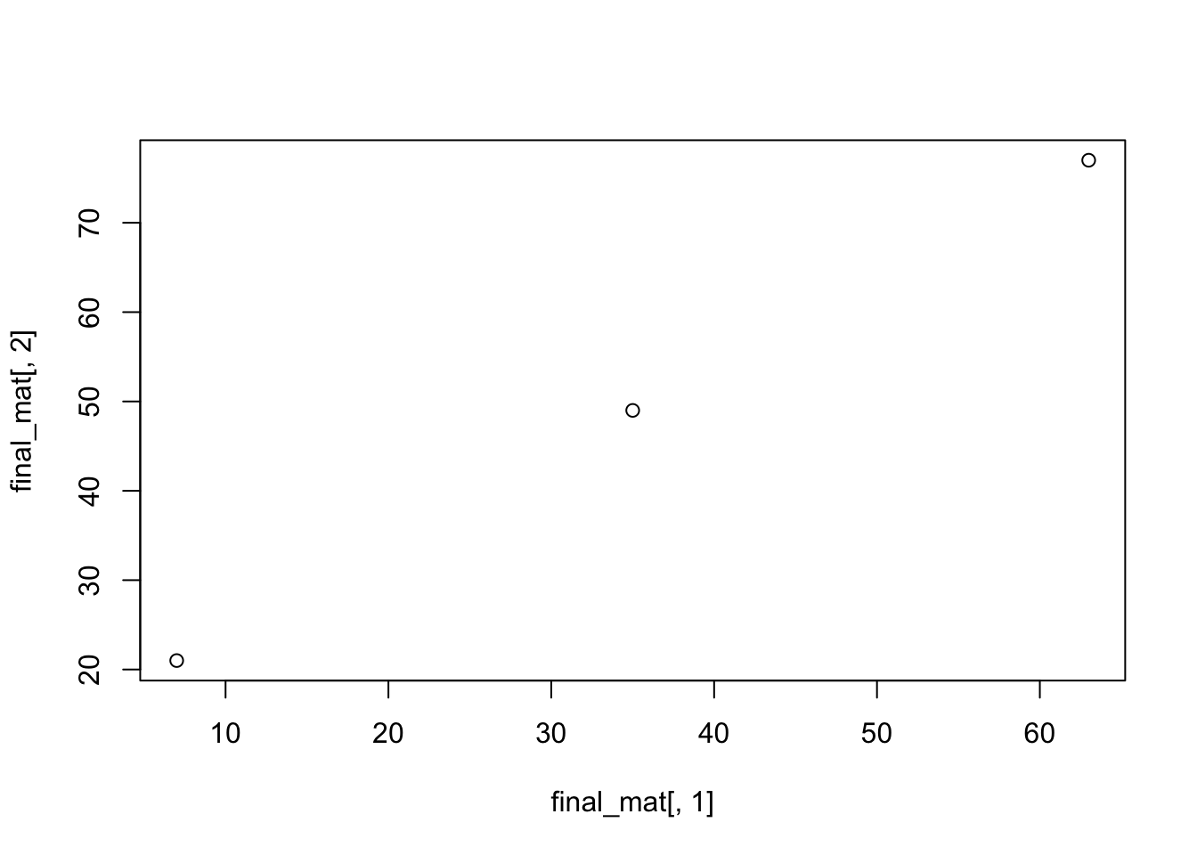
Problem 7: You want a quick estimate on how often you will win the dice game craps on the first roll. You do this by constructing 500 random rolls (2 dice/roll) and looking at the results. Use the sample function to sample the numbers 1 to 6 with replacement 1000 times, naming this vector “dice”. Take this vector and make it into a matrix named “pairs” with 2 columns and 500 rows, simulating the 500 rolls. Make a new vector summing the first and second columns named “rolls”. If 7 and 11 are the two rolls for victory on the first roll, estimate the probability of winning from your 500-roll sample. Hint: The function table might be useful in this problem.
For-loops
Often in statistical genetics you may need to repeat something several times. For example, collating results over several replicates may require a for-loop that stores the results in an array.
To illustrate the point, let’s consider a simple example. Suppose we’d like to learn how the sample mean (\(\bar{X}\)) of 50 iid standard normal random variables, \(X_1, \cdots, X_{50} \sim N(0, 1)\), behaves by simulation. To obtain one sample mean, we need to first draw 50 samples, \(X_1, \cdots, X_{50}\), from standard normal, and then calculate the sample mean as \(\bar{X} = \frac{1}{n} \sum_i X_i\). So, to obtain multiple copies of the sample mean, we need to repeat the above procedure multiple times. Let’s look at how we could implement it in R using for-loop (here we intent to obtain 1000 copies of sample mean).
- Create an empty vector of length 1000 named “sample_means”. We will fill this with sample means obtained in each replication.
- For each replication
- 2.1) Draw 50 samples
- 2.2) And calculate sample mean
- Look at “sample_means” using
summaryfunction
- Look at “sample_means” using
nrepeat = 1000
nsample = 50
sample_means <- rep(NA, nrepeat)                # Step 1
for (i in 1:nrepeat){
  samples_i = rnorm(nsample, mean = 0, sd = 1)  # Step 2.1
  sample_means[i] = mean(samples_i)             # Step 2.2
}
summary(sample_means)                           # Step 3
## Min. 1st Qu. Median Mean 3rd Qu. Max.
## -0.3990160 -0.1014323 0.0005884 -0.0008194 0.0935761 0.5137038Problem 8: How would you write a command to take the standard deviation of all elements in “sample_means” vector? Is it close to what you would expect?
Installing and loading packages
Many of the functions you may need in R may not be pre-installed. Luckily, it is very easy to install and load them, especially in RStudio. One package that is suggested for more aesthetic plotting is “ggplot2”. It is easy install and load this package, first install the package by navigating to the packages tab in the bottom right window of RStudio and click the “Install Packages” button. Then, follow the code below to load the package. Alternately, you can use the install.packages function with the name of the desired package:
library(ggplot2)You can do this with any package and can also look through all of your installed packages in RStudio to see what is loaded and not loaded already. Occasionally, you may need to install “dependencies”, which are required packages to run a specific package. Checking the box next to a package in RStudio is equivalent to using the library command.
Introduction to ggplot2
Although the standard plotting introduced in Section 2.4 will accomplish all of your plotting needs, many people prefer the aesthetics and functionality of plotting in ggplot2. We will do a very basic introduction here, just to demonstrate the syntax.
Let’s use dataset called iris available in R.
head(iris, 2)## Sepal.Length Sepal.Width Petal.Length Petal.Width Species
## 1 5.1 3.5 1.4 0.2 setosa
## 2 4.9 3.0 1.4 0.2 setosaIn short, it is giving you four measurements in three types of iris.
To learn more about the dataset, you can type ?iris in R console.
Now that we have our dataset “iris”, we can use this for our basic introduction to ggplot2. First, let’s try to just plot the first two columns (x and y coordinates) using qplot, a function made for very basic plotting in ggplot2. Follow the following steps to generate plots:
plot1 <- ggplot(iris) + geom_point(aes(x = Sepal.Length, y = Petal.Length))
plot1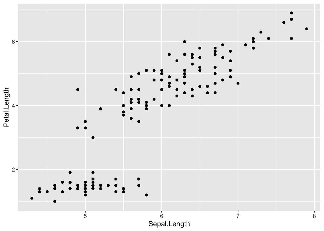
plot2 <- ggplot(iris) + geom_point(aes(x = Sepal.Length, y = Petal.Length, color = Species))
plot2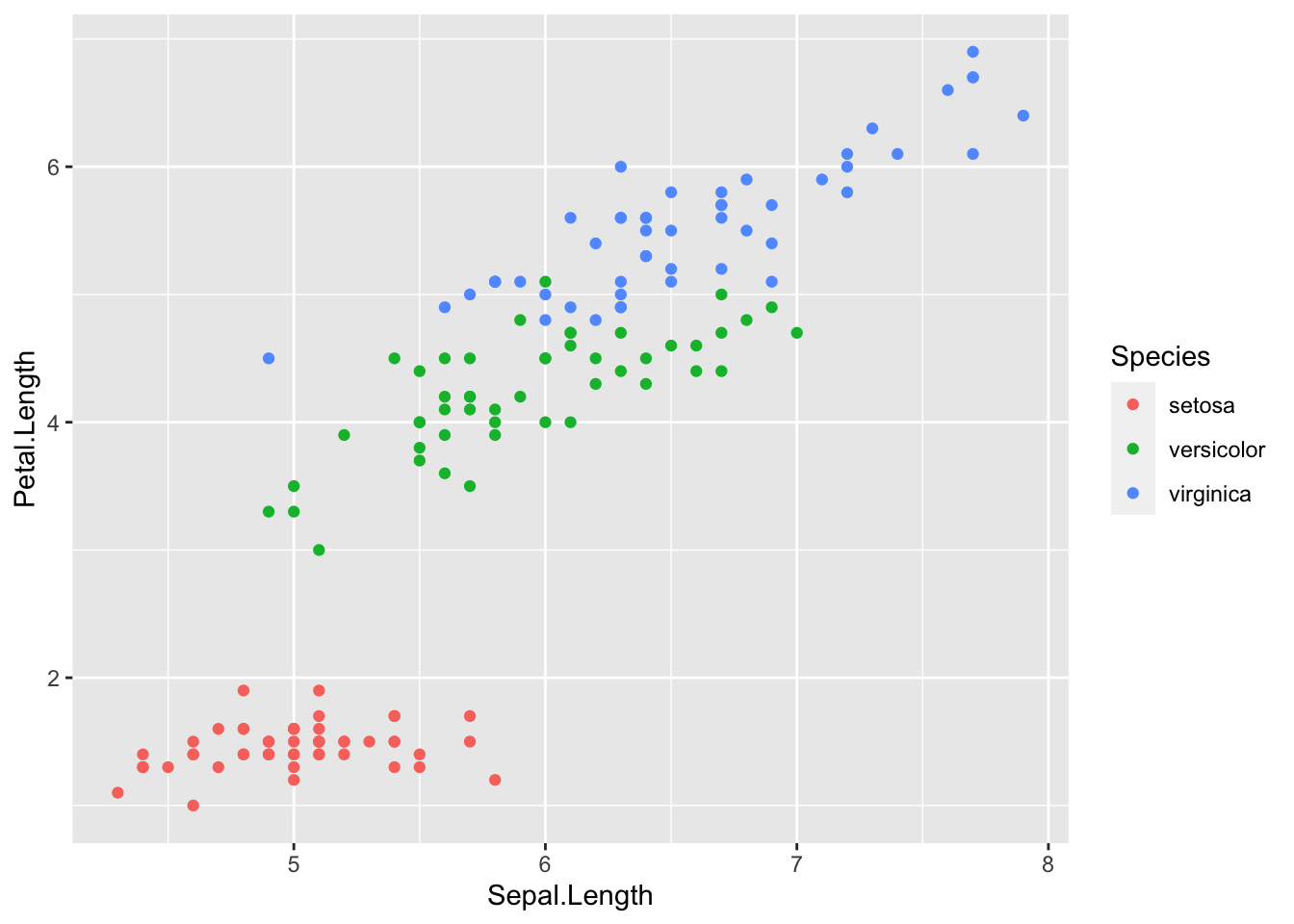
plot3 <- ggplot(iris) + geom_point(aes(x = Sepal.Length, y = Petal.Length, color = Species), alpha = 0.5)
plot3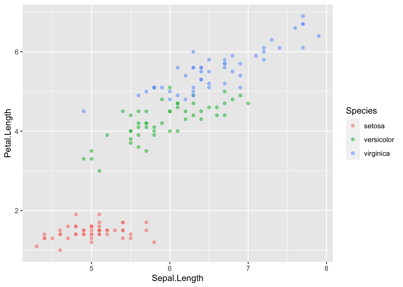
Notice a couple things here.
- To color the points by the “third”Species" column, that is simply added to the function via the “color” argument.
- When there are many dots, sometimes it is helpful to make them semi-transparent so that density is easier to see. This is done via the “alpha” argument, and ranges from 0 (transparent) to 1 (opaque).
- Notice the coloring could be on a spectrum if the variable is numeric. For example, follow the commands below to color by Sepal.Width:
plot4 <- ggplot(iris) + geom_point(aes(x = Sepal.Length, y = Petal.Length, color = Sepal.Width))
plot4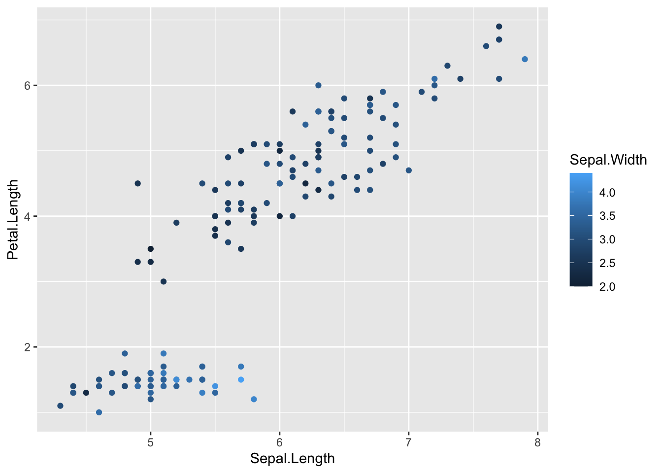
Problem 9: Take a look at the help page of geom_boxplot and make a boxplot where “Species” is on x-axis and “Petal.Length” is on y-axis