Created by Max Winston, modified by Charles Washington III, Ankeeta Shah, and Yanyu Liang
(from HGEN47100 course material)
Before getting started, please download data from the Box link here. For your convenience, we have a copy of the data folder at /project2/hgen47100/data/lab2 on midway.
wget https://uchicago.box.com/shared/static/30h5kju8ggui94whfbz0prjn3x4dvtag.gz -O lab2.tar.gz
tar xvf lab2.tar.gz
Tranferring data between midway and local machine. Unix users are recommended to use scp or rsync. Windows users can use WinSCP or equivalent. For our purpose, our files are not sensitive and small in general. An alternative approach is to login to midway Desktop using ThinLinc and send the data as an email.
This lab section is dedicated to learning how to manipulate the appropriate files in a command-line program named PLINK (to run whole-genome association and population-based linkage analysis). By the end of this lab, you should be able to:
- Know about PED and BED files
- Run GWAS using PLINK for both discrete and continuous phenotypes
- Account for covariates in GWAS run
- Visualize GWAS outputs generated by PLINK
The Basics of PLINK
Basic Commands and Options
PLINK is a comprehensive program with an enormous range of functionalities and options. We will introduce some basic commands here to get you started, but inevitably, you will want to visit the PLINK documentation.
Regarding the PLINK version, you may see three versions available currently (Jan 2020). They are: v1.07, v1.9, and v2. PLINK v1.9 and v2 are under active development whereas v1.07 is not. Throughout this lab, we will use PLINK v1.9. The reason is two-fold: 1) v1.9 has many enhancements over v1.07 and it is still getting even better; 2) as a fast growing field, new features are actively incorporated into newer version.
In the following, we list some commonly used commands in PLINK. To get to know more about how to use PLINK v1.9, here is the online documentation.
| Command | Description |
|---|---|
| make-bed | Converts a PED file to a BED file. |
| missing | Generates summary statistics on missing data. |
| freq | Generates summary statistics on allele frequencies. |
| assoc | Runs a basic genome-wide association analysis (on discrete or continuous trait). |
In addition to the commands which generate files on their own, the following basic options are important. In any analysis, it is important to perform quality control on the input data (so that we reduce the chance to be placed at “garbage in, garbage out” situation). And equally importantly, we should report how the QC is done in the manuscript (e.g. what thresholds/limits are used to filter out outliers, etc). Often, you may want to use many values to explore whether the perceived association or relationship is robust to your a priori limits.
| Option | Description |
|---|---|
| mind | Upper limit for the rate of SNPs missing for individual. |
| geno | Upper limit for the rate of individuals missing at a given SNP. |
| hwe | Lower limit for deviation from Hardy-Weinberg Equilibrium (unit = p-value). |
| maf | Lower limit for Minor Allele Frequency (MAF). |
| chr | Limits to a single chromosome. |
| within | Allows for stratified analysis. |
| adjust | Reports adjusted significance values for an association. |
PLINK syntax
PLINK syntax follows basic Unix style commands seen in Lab 1. However, one notable element of the syntax is that PLINK generally takes the file name without extension. For example, one of the first steps in PLINK is to make a BED file from a PED file. In such an example, a command could be:
plink --file hapmap1 --make-bed --out hapmap1Here, we are calling the PLINK command and providing the root for the input file “hapmap1”, commanding PLINK to make a BED file (“–make-bed”), and naming an output “hapmap1-out.bed”.
PED files
It is helpful to know the correct format for PED files in case you want to troubleshoot or design an automated script to modify an existing PED file. All PED files are white-space (space or tab) delimited files, arranged such that the first six columns are mandatory:
- 1) Family ID
- 2) Individual ID
- 3) Paternal ID
- 4) Maternal ID
- 5) Sex (1 = male, 2 = female; other = unknown)
- 6) Phenotype
All IDs are alphanumeric, and a PED file must have only 1 phenotype in the sixth column, and may be quantitative or qualitative. Every two columns after the first six are genotypes of SNPs listed in .map file in the same order. These SNPs should be biallelic so that can be represented by numbers or letters (1,2,3,4 or A,T,G,C), as long as 0 is not used (this is default for missing data). So, each of the two columns represent the genotype of a biallelic locus. For instance, 7th and 8th column are allele calls for the first variant in the .map file. Therefore, the number of columns in any PED file is equal to 2 times the number of SNPs (genotypic data) plus the leading six columns.
If you’d like to get to know more on PED format, PLINK documentation has detailed description at here. More importantly, there are many more formats that could be input or generated by PLINK. Whenever you encounter a new format, you can get to know about it using PLINK documentation File formats page.
Although BED files (binary PED files) are often used for analyses to reduce computational time, they are much harder to work with since they are in binary format, and thus generally modifications are made to PED files and then they are then converted to BED files using the command in Section 1.2.
Basic Operations (HapMap Example)
Download and unzip dataset and load PLINK
To begin, we will start with the dataset included with the standard PLINK download. This dataset includes randomly selected genotypes (~80,000 autosomal SNPs) from 89 Asian HapMap individuals. In order to download this data for this lab, navigate to your directory on the cluster, and use the following command to download the zipfile:
cd ~/Downloads/tempo/
curl zzz.bwh.harvard.edu/plink/hapmap1.zip > hapmap1.zip
Next, create a new directory, unzip the file you downloaded, and place the contents in that directory. If you have trouble doing this, you can refer to some of the basic commands from Lab 1.
You should note that this file is a .zip file rather than a .tar file. As such you should use the unzip command instead of the tar command to access the contents.
unzip hapmap1.zipNow that we have our dataset, we need to access PLINK, the software we’ll be using for this lab. Last week we download the program we needed from the internet, but this week we’ll be accessing the program directly from the cluster. Clusters, particularily those that service genetics and genomic research at institutions, often come with many programs built in. These programs are available to all users and prevents them from needing to download multiple programs to their individual machines. View the versions of PLINK available to you and load the specified version of PLINK.
- 1) Look at the programs available for you to load
- 2) Specifically look at the version of plink available to you
- 3) Load the current version of plink for you to use
module avail                   ##Step 1
module avail plink             ##Step 2
module load plink/1.90b6.9     ##Step 3
Sidenote: the midway cluster has a number of other software packages already pre-installed. For future reference, if you want to determine what packages / whether a specific package is already installed on the cluster:
module avail #to list all packages installed on the cluster
module avail <insert_package_name> #to check if a specific package is installed
Converting PED files to BED files
Now that you have access to PLINK, this next command will convert the example hapmap1 PED file to a BED file. Make sure these commnads are entered in the same directory where the hapmap files are located. Note that once you have converted to a BED file, the input command becomes bfile instead of file. Type the following to convert your PED to a BED file:
plink --file hapmap1 --make-bed --out hapmap1This command should have converted your input file (hapmap1.ped) into a binary PED file (hapmap1.bed). Check for the new file by looking through your directory. You may notice that there are now two other types of files in the directory (hapmap1.bim and hapmap1.fam). The .bim file is a revised mapping file and the .fam file is the first six columns of the PED file. Although it is fine to extract data from these files, people usually do not edit them manually.
Generating statistics on missing data
Often, datasets may have missing data, and it is helpful to know some general statistics on this missing data. To generate these stats, type the following:
plink --bfile hapmap1 --missing --out miss_statThis command will create miss_stat.lmiss and miss_stat.imiss files, summarizing the per SNP and per individual rates of missing data, respectively. Open take a look at these files in Terminal to check formatting.
Problem 1
What are the columns for the two files generated (.lmiss & .imiss)?
Try the following command to get some basic summary data on the files:
wc miss_stat.imissProblem 2
What do the different numbers returned from the command above correspond to (hint: man)? How many SNPs are in this dataset?
Generating statistics on allele frequencies
For most analyses it is important to know the minor allele frequencies (MAF) for any individual SNP, as you may want to restrict the analysis to SNPs with MAF above a particular value. To generate a file with all SNPs and the MAF, type the following command:
plink --bfile hapmap1 --freq --out freq_statProblem 3
What are the different columns in the file generated (freq_stat.frq)? What do you think they mean?
Using PLINK options to perform QC
Basic QC
There are a number of options within PLINK to modify your input files for your desired analysis. Four of the most common options for quality control are
- Removing individuals with high missingness (–mind);
- Removing SNPs with low MAF (–maf);
- Removing SNPs with high missingness (–geno);
- Removing SNPs that deviate significantly from Hardy-Weinberg Equilibrium (–hwe).
Although you can modify these options however you like, let’s apply some “reasonable” cut-offs to the HapMap dataset. Try the following command to apply our quality control:
plink --file hapmap1 --make-bed --mind 0.05 --maf 0.01 --geno 0.05 --hwe 0.05 --out hapmap1_QC1Problem 4
Given your knowledge of the options and PLINK syntax, translate the above command into a description of our quality control.
Problem 5
Use the commands learned in Section 1.4 to generate statistics on missing data and allele frequencies for hapmap1_QC1. Make sure not to name them the same thing as the previously generated statistic files. How are the files generated from hapmap1 and hapmap1_QC1 different? Are the number of individuals the same after our quality control? The number of SNPs?
User-directed QC
Sometimes rather than setting simple threshold values, the user may want to provide a specific list of SNPs or individuals to use or to exclude. For instance, we only want to keep individuals having signed study consent or we want to exclude SNPs which are labelled as bad SNPs by our collaborators.
For SNPs, it is possible to exclude SNPs specified in a list (–exclude), or only use those SNPs in the list (–extract). For individuals, it is possible to remove individuals specified in a list (–remove), or only use those individuals in the list (–keep). It is important to note that the file should be a simple text file, with the name of a single SNP on each line.
We’ll use the badSNPs.txt text file in the data folder you’ve downloaded. For your convenience, the same copy of file is on midway2 at the path: /project2/hgen47100/data/lab2/badSNPs.txt.
Using a list of questionable SNPs (badSNPS.txt) we can remove them from our dataset:
# on midway2
plink --file hapmap1 --make-bed --exclude /project2/hgen47100/data/lab2/badSNPs.txt --mind 0.05 --maf 0.01 --geno 0.05 --hwe 0.05 --out hapmap1_QC2

## on your mac
plink --file hapmap1 --make-bed --exclude lab2/badSNPs.txt --mind 0.05 --maf 0.01 --geno 0.05 --hwe 0.05 --out hapmap1_QC2
Problem 6
Generate statistics for this new BED file. How many SNPs are there in the hapmap1_QC2 dataset?
Running basic associations
After quality control, most frequently you will run some sort of association on your trimmed dataset. In our HapMap1 dataset, the phenotype embedded in the hapmap1_QC2 file (let’s call it Disease XXX) was actually generated to specifically associate with a particular genetic variant (rs2222162) in a probabilistic framework. Let’s see if we can find it with a basic association test. Basic association tests can easily be run with the following command:
plink --bfile hapmap1_QC2 --assoc --out assoc_QC2Now that we have generated our association file assoc_QC2, let’s use some of our Unix commands we learned in Lab 1 to manipulate this file. Follow the command below to list the top ten associated SNPs in our new association file:
sort --key=9 -g assoc_QC2.assoc | headThis command should print the top ten SNPs on the screen.
Problem 7
Is the particular genetic variant (rs2222162) in the top ten associated SNPs? Does it have the most significant association?
Problem 8
Use commands we know to take this list and write it into a text file named top_ten_assoc_QC2.txt.
Other types of association, such as logistic regression, can be run just as easily. Run an association using logistic regression with the following command:
plink --bfile hapmap1_QC2 --logistic --out log_assoc_QC2Problem 9
Observe the top ten SNPs in log_assoc_QC2. How do they compare to those from assoc_QC2?
Manhattan plots
Manhattan plots are one of the most common ways of visualizing GWAS results, and are simple scatter plots where the x-axis gives the genomic coordinates and the y-axis gives the negative log of the p-value for an individual SNP. Because of the vast number of the points (SNPs), it kind of resembles the Manhattan skyline, thus the name. Although there are a number of different ways to create a Manhattan plot, today we will just use the plotting packages we have already introduced. There are also other popular packages for making Manhattan plots in R (i.e. qqman). Open R Studio, change your working directory to the data folder you downloaded. And try the following commands:
library(ggplot2)                                             ## Load package
assoc_QC2 <- read.table(                                     ## Read in data
  "~/Downloads/tempo/assoc_QC2.assoc",
  header = TRUE, stringsAsFactors = FALSE
)
assoc_QC2 <- subset(assoc_QC2, P != "NA")                    ## Trim data
#Sets a color scheme for the chromosomes w/ hex codes, these can also be coded with plaintext names (i.e. "red")
our_colors <- c("#FF0000", "#a6cee3","#0000FF","#1f78b4", "#00FF00","#b2df8a","#33a02c","#fb9a99","#91003f","#fdbf6f","#ff7f00","#cab2d6","#6a3d9a","#ffff99","#b15928","#d95f0e","#377eb8","#4d4d4d","#999999","#dd1c77","#542788","#c994c7")
#Sets the bonferroni-corrected threshold
bonferroni <- -log(0.05 / length(assoc_QC2$P))
#Plots the data with all the aesthetic and plotting options
ggplot(assoc_QC2)  +
  geom_point(aes(x = BP, y = -log(P), color = factor(CHR)), size = 2, alpha = 0.5) +
  scale_y_continuous(limits = c(0,15)) +
  geom_hline(yintercept = bonferroni, linetype = 2) +
  xlab("SNP Position (Chromosomes Ordered 1-22)") +
  ylab("Association Significance (-log(p-value))") +
  labs(color = 'Chromosome') +
  scale_colour_manual(values = our_colors)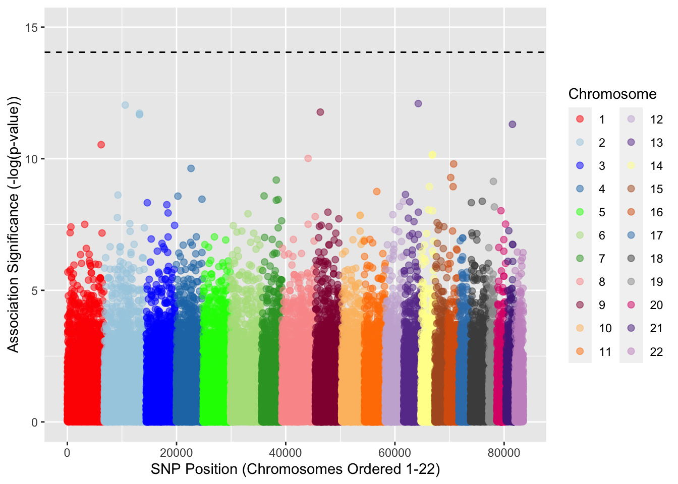
Here we have produced a Manhattan plot, with colors of the dots (SNPs) indicating the appropriate chromosomes. We have also plotted a dotted line which is a threshold for signifance after multiple-testing correction. The multiple-correction procedure we have used here is the Bonferroni correction, which is the most conservative in terms of avoiding false positives, which is why none of the SNPs are significant.
Running a Case-Control GWAS
One of the most common uses of GWAS is to explore putative associations for disease. In this section we will practice our skills with PLINK using a dataset with SNPs in a 20Mb region from a case-control GWAS of a binary phenotype (more than 5000 individuals). There is a little readme (readme_of_GAME_data.txt) which you may find useful. The input files have already been downloaded inside the data folder. It includes small GWAS file set (bed/bim/fam files), as well as the file containing covariates obtained from principal components analysis (PCA). For your convenience, you can find these files at /project2/hgen47100/data/lab2.
Throughout this section, you will be asked to run multiple PLINK commands. You will be asked to record them all in one bash script as part of the submission.
Preliminary Quality Control
Your first task is to use PLINK to remove SNPs with low call rates (>5% missingness), deviation from Hardy-Weinberg equilibrium (p < 0.001), and low minor allele frequency (MAF < 0.05). Please record the command in the bash script.
Problem 10
Provide the script you used. How many SNPs, in total, were removed and how many are left?
Logistic Regression
Test associations for this chromosome using logistic regression (–logistic) using the “–adjust” flag to conduct adjustments for multiple testing. No phenotype file needs to be specified because case-control status is in the .fam file, Please record the command in the bash script
Problem 11
Look through the most significant SNPs in the logistic association results file. What is the most significant SNP? What is the p-value? (Make sure you look at the .assoc.logistic.adjusted file’s Bonferroni-corrected value (BONF) as this gives you the corrected significance).
Now run the same command adjusting for five principal components (PCs) representing ancestry using the “–covar” flag for the 5 ancestral PC file and the “hide-covar” flag. Don’t worry too much about correcting for ancestry using PCs, we will get into much more detail on this in a later lab. Please record the command in the bash script
Problem 12
What is the most significant SNP now? What is the p-value?
Problem 13
Are the results the same from Problem 11 and Problem 12? Did correcting for ancestry do anything?
Problem 14 Make two Manhattan plots by importing the two .assoc.logistic files (not the adjusted versions) into R and using some of the code above (you’ll need to move them from the cluster to your local environment). Keep in mind that the length of the file is different from the previous Manhattan plot, so you may need to change the significance threshold as well as the data used. What are the main differences between the two plots?
Creating a Locuszoom Plot
Locuszoom plots have the same basic structure as Manhattan plots, however, they are useful in that they include additional information such as gene location, r-squared values (LD), and estimated recombination rates. Once you have generated your logistic association file (the one using the 5 PCs) from Section 2.2 and identified the top SNP from this association, it is very easy to navigate to the Locuszoom website and create the plot.
Create a locuszoom plot using the web server here. Use the significance reported in the .logistic file (not the .logistic.adjusted file) from section 2.2. (once again, you’ll need to move the file from the cluster to your local environment).
The website recognizes a SNP by genomic position along with the reference/alternative alleles. But the current .logistic file does not includes non effect allele. To fix this issue, please refer to example_rscript_to_convert_plink_assoc_to_locuszoom_input.R in the data folder to see one possible work-around.
After uploading the GWAS results, you will hit button “submit” which will submit a job to server to generate the locus zoom plots. Once the job is finished, you will be noticed by email with the link to report. In the report page, the link “region plot” directs you to the locuszoom plot. The color of each point indicates the pairwise correlation of that SNP with the focal SNP (which we entered as the most highly associated SNP). Additionally, the blue line in the background demonstrates the estimated recombination rate (cM/Mb) from the much larger HapMap dataset external to our Case-Control dataset.
Problem 15
Why do you think many of the SNPs surrounding the focal SNP are colored more red-ish (i.e. are more correlated)? Do you notice any pattern between the color of these points and the background recombination rate?
Assessing multiple association signals in this region
Often, you may want to know whether there are other significant association signals conditional upon identification of a highly-associated SNP (such as the one you identified in Section 2.2). To determine if there are multiple association signals in this region, run the logistic with covariates again using the “–condition rsXXXX”" flag to adjust for the top SNP. Please record the command in the bash script
Problem 16
Use locuszoom to plot the -log10 P-values from the new analysis. Show the plots for both the unconditioned (the very first locuszoom plot) and the conditioned files (for region 13:73666628-74166628).
Problem 17
Interpret the results of the two plots by writing 1-2 sentences for each.