Learning objectives
- recall definition of p-value
- calculate p-value analytically and empirically for a simple example
- build intuition about p-values when multiple testing is performed via simulations
- recognize the need for multiple testing correction
- present methods to correct for multiple testing
- Bonferroni correction
- FDR (false discovery rate)
Review p-value with normal example
Let’s sample one value Z from the standard normal distribution
set.seed(8050151)
z1 = rnorm(1, mean=0, sd=1)
z1
## [1] -0.6089123Let’s calculate now the p-value of this observation. Recall that the p-value is the probability that we will draw a sample as extreme as the observed value under the null distribution (i.e. when the null distribution is the true distribution).
We can calculate that number exactly for this simple case: \[\begin{align} p &= \text{pnorm}(-abs(z_1)) + 1 - \text{pnorm}(abs(z_1))\\ &= 2 \cdot \text{pnorm}(-abs(z_1)) \end{align}\]
The theoretical p-value is 0.5425825. So we do not reject the null hypothesis. When there is only one test being performed, the rule of thumb is that the p-value should be smaller than 0.05 to reject the null hypothesis.
We can calculate the p-value empirically as follows:
We draw 10,000 samples from the standard normal distribution and calculate the proportion of draws that fall below \(-|z_1|\) or above \(|z_1|\)
nsim = 10000
zvec = rnorm(nsim, mean=0, sd=1)
hist(zvec)
abline(v=c(-abs(z1),abs(z1)))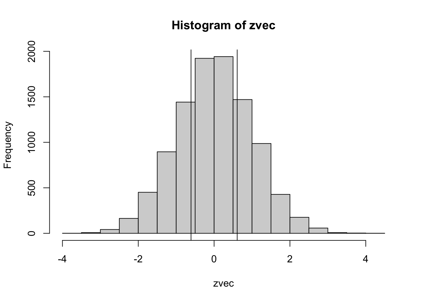
p_emp = sum(abs(zvec)>abs(z1)) / nsimSo, the p-value of our observation \(z_1\) is 0.5432, which is pretty close to the analytical value we calculated above: 0.5425825.
Motivate the need for multiple testing correction
We will simulate \(Y = X \cdot \beta + \epsilon\), a standard linear model. We start by simulating a vector of \(X\) and \(\epsilon\).
## set seed to make simulations reproducible
set.seed(20210108)

## define some parameters for the simulation
nsamp = 100
beta = 2
h2 = 0.1 ## we want X to explain 10% of the variation in Y
sig2X = h2
sig2epsi = (1 - sig2X) * beta^2
sigX = sqrt(sig2X)
sigepsi = sqrt(sig2epsi)

## simulate normally distributed X and epsi
X = rnorm(nsamp,mean=0, sd= sigX)
epsi = rnorm(nsamp,mean=0, sd=sigepsi)

## generate Yalt (X has an effect on Yalt)
Yalt = X * beta + epsi

## plot Yalt vs X
plot(X, Yalt, main="Yalt vs X")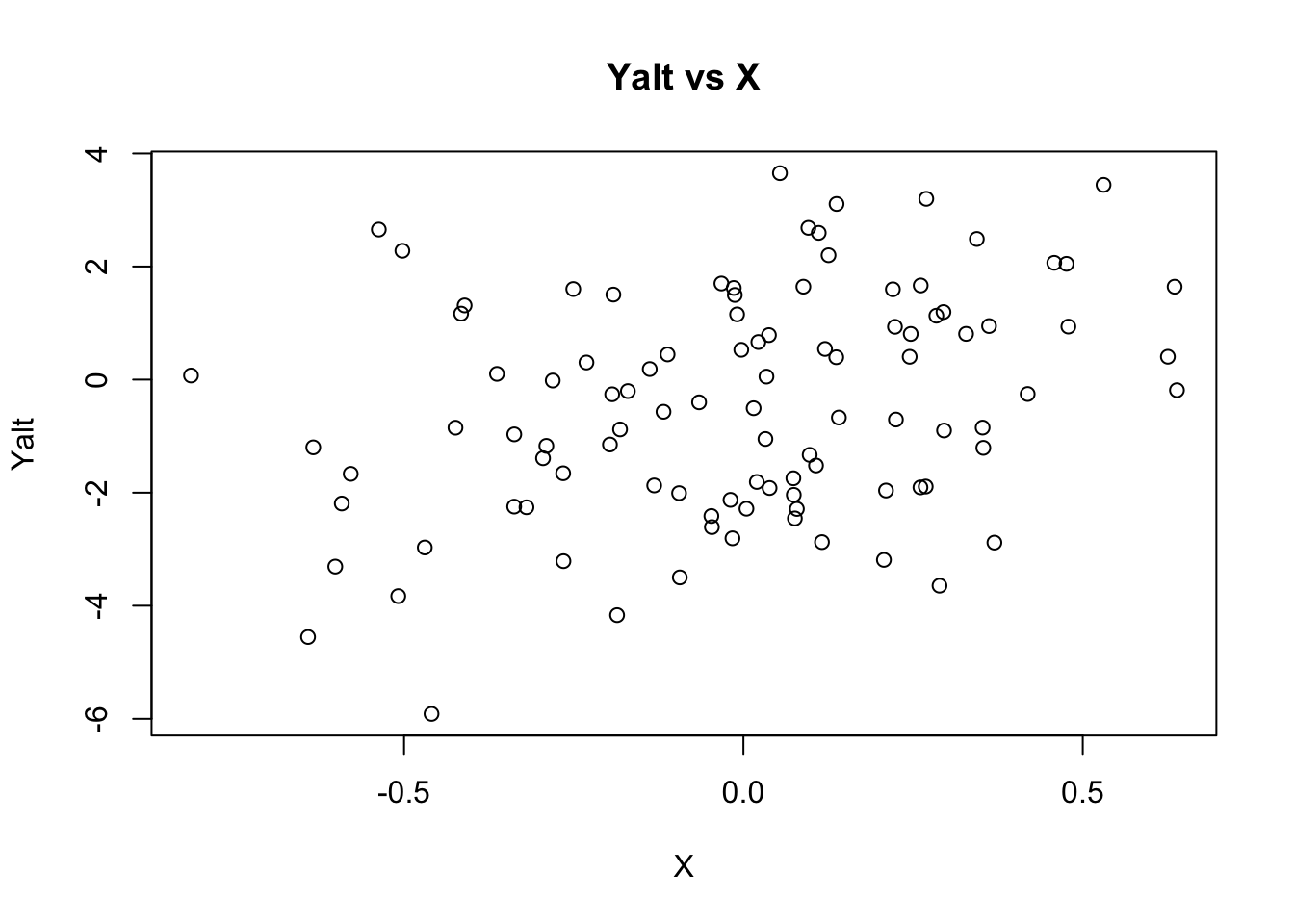
## generate Ynull (X has no effect on Ynull)
Ynull = rnorm(nsamp, mean=0, sd=beta)

## plot Ynull vs X
plot(X, Ynull, main="Ynull vs X")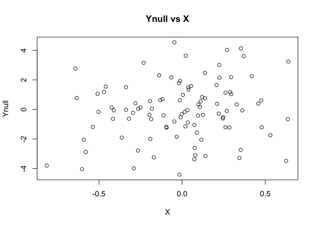
## test association between Ynull and X
summary(lm(Ynull ~ X))
##
## Call:
## lm(formula = Ynull ~ X)
##
## Residuals:
## Min 1Q Median 3Q Max
## -4.3548 -1.1589 0.0782 1.3735 4.6291
##
## Coefficients:
## Estimate Std. Error t value Pr(>|t|)
## (Intercept) -0.0395 0.1951 -0.202 0.840
## X 1.0095 0.6240 1.618 0.109
##
## Residual standard error: 1.95 on 98 degrees of freedom
## Multiple R-squared: 0.02601, Adjusted R-squared: 0.01607
## F-statistic: 2.617 on 1 and 98 DF, p-value: 0.1089what’s the p-value of the association?
is the p-value significant at 5% significance level?
what about Yalt and X?
summary(lm(Yalt ~ X))##
## Call:
## lm(formula = Yalt ~ X)
##
## Residuals:
## Min 1Q Median 3Q Max
## -4.5453 -1.4809 0.1231 1.2189 4.1808
##
## Coefficients:
## Estimate Std. Error t value Pr(>|t|)
## (Intercept) -0.4244 0.1891 -2.244 0.0271 *
## X 2.0521 0.6050 3.392 0.0010 **
## ---
## Signif. codes: 0 '***' 0.001 '**' 0.01 '*' 0.05 '.' 0.1 ' ' 1
##
## Residual standard error: 1.89 on 98 degrees of freedom
## Multiple R-squared: 0.1051, Adjusted R-squared: 0.09595
## F-statistic: 11.51 on 1 and 98 DF, p-value: 0.001001what’s the p-value of the association?
is the p-value significant at 5% significance level?
Distribution of the p-values - mixture of null and alternative
We want to run 10000 times this same regression, so here we define a function fastlm that will get us the p-values and regression coefficients, a bit faster than the built-in lm function.
fastlm = function(xx,yy)
{
  ## compute betahat (regression coef) and pvalue with Ftest
  ## for now it does not take covariates

  df1 = 2
  df0 = 1
  ind = !is.na(xx) & !is.na(yy)
  xx = xx[ind]
  yy = yy[ind]
  n = sum(ind)
  xbar = mean(xx)
  ybar = mean(yy)
  xx = xx - xbar
  yy = yy - ybar

  SXX = sum( xx^2 )
  SYY = sum( yy^2 )
  SXY = sum( xx * yy )

  betahat = SXY / SXX

  RSS1 = sum( ( yy - xx * betahat )^2 )
  RSS0 = SYY

  fstat = ( ( RSS0 - RSS1 ) / ( df1 - df0 ) )  / ( RSS1 / ( n - df1 ) )
  pval = 1 - pf(fstat, df1 = ( df1 - df0 ), df2 = ( n - df1 ))
  res = list(betahat = betahat, pval = pval)

  return(res)
}
Simulate p-values under the null and alternative
nsim = 10000

## simulate normally distributed X and epsi
Xmat = matrix(rnorm(nsim * nsamp,mean=0, sd= sigX), nsamp, nsim)
epsimat = matrix(rnorm(nsim * nsamp,mean=0, sd=sigepsi), nsamp, nsim)

## generate Yalt (X has an effect on Yalt)
Ymat_alt = Xmat * beta + epsimat

## generate Ynull (X has no effect on Ynull)
Ymat_null = matrix(rnorm(nsim * nsamp, mean=0, sd=beta), nsamp, nsim)

## let's look at the dimensions of the simulated matrices

dim(Ymat_null)
## [1] 100 10000dim(Ymat_alt)## [1] 100 10000## Now we have 10000 independent simulations of X, Ynull, and Yalt
## give them names so that we can refer to them later more easily
colnames(Ymat_null) = paste0("c",1:ncol(Ymat_null))
colnames(Ymat_alt) = colnames(Ymat_null)
## Let's run 10000 linear regressions of the time Ynull = X*b + epsilon, to do this in a reasonable amount of time, we will use the fastlm function we defined above.
pvec = rep(NA,nsim)
bvec = rep(NA,nsim)
for(ss in 1:nsim)
{
fit = fastlm(Xmat[,ss], Ymat_null[,ss])
pvec[ss] = fit$pval
bvec[ss] = fit$betahat
}
summary(pvec)## Min. 1st Qu. Median Mean 3rd Qu. Max.
## 0.0000021 0.2438476 0.4903663 0.4935828 0.7401156 0.9998408hist(pvec,xlab="p-value",main="Histogram of p-values under Null")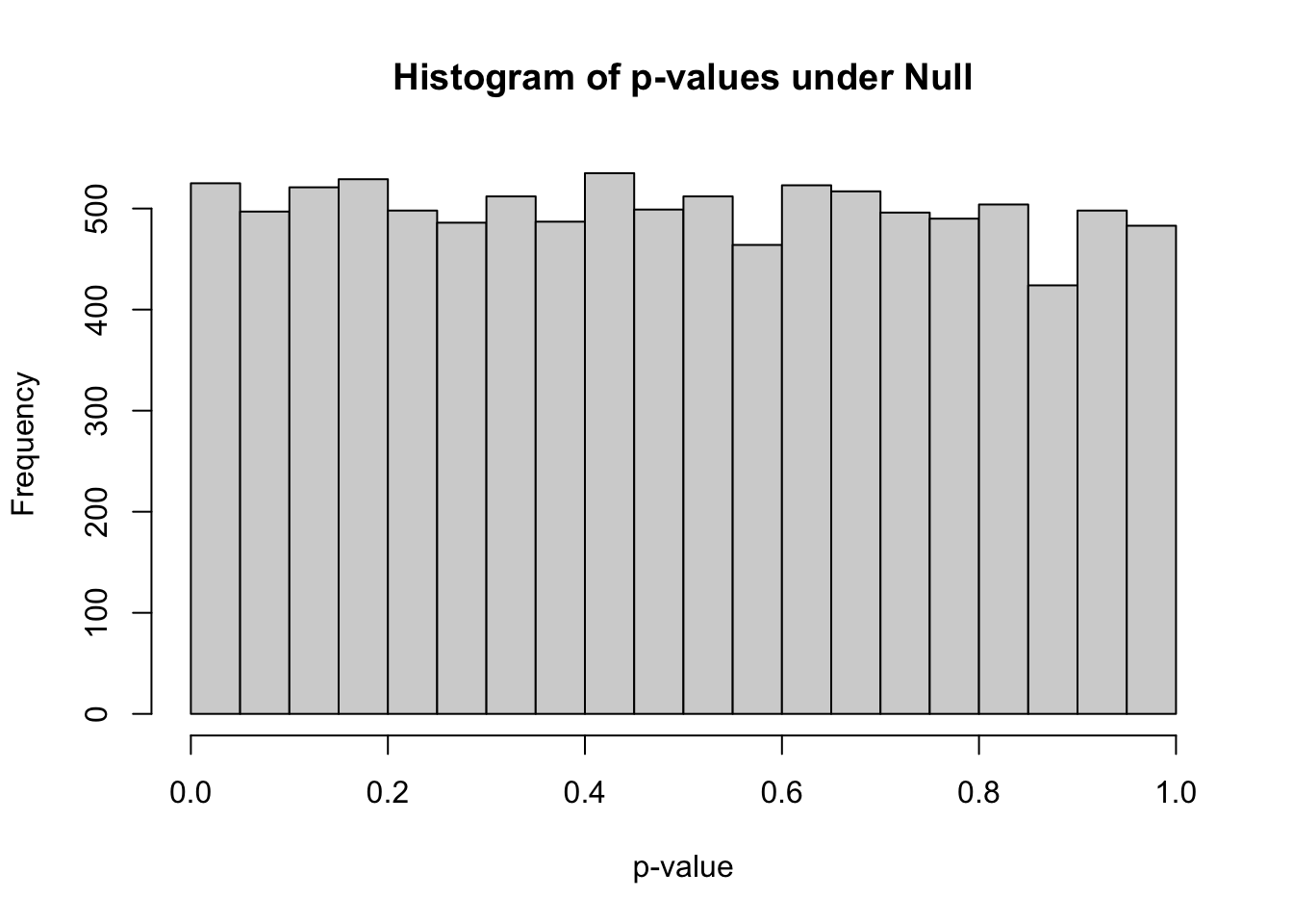
- how many simulations under the null yield p-value below 0.05? What percentage is that?
Note1
sum(pvec<0.05)## [1] 525mean(pvec<0.05)## [1] 0.0525how many simulations under the null yield p-value < 0.20?
Why do we need to use more stringent significance level when we test many times?
So it is clear that when we are performing thousands of tests, we cannot just use 0.05 as the threshold of significance, because that will give us 5% of the tests will achieve significance when the null hypothesis is true, i.e. 5% will be false positives, and the probability of calling at least one null case significant approaches 1 as the number of tests increases.
A common way to address the multiple testing issue is by using the Bonferroni correction (it controls the familywise error rate FWER). This uses a much more stringent significance threshold for each test to keep overall false positive at 5%.
Bonferroni correction
Bonferroni correction requires the threshold for significance of the p-value is obtained by dividing by the number of tests. So typically
\[\frac{0.05}{\text{total number of tests}}\]
what’s the Bonferroni threshold for significance in this simulation?
how many significant associations did we find?
BF_thres = 0.05/nsim
## Bonferroni significance threshold
print(BF_thres)
## [1] 5e-06## number of Bonferroni significant associations
sum(pvec<BF_thres)## [1] 1## proportion of Bonferroni significant associations
mean(pvec<BF_thres)## [1] 1e-04GWAS significance threshold

GWAS Figure
The consensus value for calling a GWAS hit significant is \(5\cdot 10^{-8}\). How many tests are we correcting the usual 0.05 threshold?
Current GWAS have typically 10 million SNPs but we still use \(5\cdot 10^{-8}\). What do you think is the justification?
Mix of Ynull and Yalt
Let’s see what happens when we add a bunch of true associations in the matrix of null associations. This is a more likely scendario in a GWAS, some SNPs are causally affecting the trait (alternative hypothesis is true for these SNPs) whereas other SNPs will have no effect on the trait (null hypothesis is true).
prop_alt=0.20 ## define proportion of alternative Ys in the mixture
selectvec = rbinom(nsim,1,prop_alt)
names(selectvec) = colnames(Ymat_alt)
selectvec[1:10]
## c1 c2 c3 c4 c5 c6 c7 c8 c9 c10
## 1 0 0 0 1 1 0 0 0 1Ymat_mix = sweep(Ymat_alt,2,selectvec,FUN='*') + sweep(Ymat_null,2,1-selectvec,FUN='*')
## Ymat_mix should have Yalt for columns that have 1's in selectvec and Ynull where selectvec==0
print(head(Ymat_mix[,1:10]),2) ## use 2 decimals## c1 c2 c3 c4 c5 c6 c7 c8 c9 c10
## [1,] 1.72 -0.4 -1.06 2.49 0.6637 -0.021 -0.024 4.177 -2.39 2.46
## [2,] 0.72 -2.1 -0.64 0.30 1.7522 -1.704 1.457 -0.085 -1.67 0.33
## [3,] -1.58 1.4 2.55 0.65 -2.0064 -0.427 3.817 -2.514 -1.54 1.90
## [4,] 1.06 1.1 -1.99 0.32 2.0433 0.792 0.255 -0.567 -1.43 0.06
## [5,] -1.55 -3.9 -0.53 1.45 -0.0054 1.736 -0.681 1.339 -0.68 -0.55
## [6,] 2.71 1.6 -0.83 -1.70 -1.1723 0.882 -1.150 4.442 -2.68 -3.95print(selectvec[1:10])## c1 c2 c3 c4 c5 c6 c7 c8 c9 c10
## 1 0 0 0 1 1 0 0 0 1print("subtract Ymat_alt")## [1] "subtract Ymat_alt"print(head(Ymat_mix[,1:10] - Ymat_alt[,1:10]),2)## c1 c2 c3 c4 c5 c6 c7 c8 c9 c10
## [1,] 0 -1.33 -0.094 3.130 0 0 2.0 2.46 -0.96 0
## [2,] 0 -2.59 3.562 1.311 0 0 1.4 4.67 -1.76 0
## [3,] 0 1.05 0.273 -0.045 0 0 4.4 -3.20 3.70 0
## [4,] 0 3.29 -0.959 5.577 0 0 -1.8 -0.22 -0.71 0
## [5,] 0 -3.81 -1.331 3.413 0 0 -3.4 0.55 -4.43 0
## [6,] 0 -0.73 -0.381 -3.416 0 0 -1.7 5.82 -3.14 0print("subtract Ymat_null")## [1] "subtract Ymat_null"print(head(Ymat_mix[,1:10] - Ymat_null[,1:10]),2)## c1 c2 c3 c4 c5 c6 c7 c8 c9 c10
## [1,] 2.91 0 0 0 1.62 -0.69 0 0 0 0.47
## [2,] -1.41 0 0 0 2.63 0.20 0 0 0 3.51
## [3,] -2.19 0 0 0 -0.99 1.64 0 0 0 2.77
## [4,] 0.57 0 0 0 5.23 3.09 0 0 0 -0.50
## [5,] -4.57 0 0 0 -0.68 -1.97 0 0 0 2.19
## [6,] 3.57 0 0 0 -4.26 2.85 0 0 0 -4.06## Q: how many columns have true effect and how many have null effects
sum(selectvec)## [1] 2004mean(selectvec)## [1] 0.2004## run linear regression for all 10000 phenotypes in the mix of true and false associations, Ymat_mix
pvec_mix = rep(NA,nsim)
bvec_mix = rep(NA,nsim)
for(ss in 1:nsim)
{
fit = fastlm(Xmat[,ss], Ymat_mix[,ss])
pvec_mix[ss] = fit$pval
bvec_mix[ss] = fit$betahat
}
summary(pvec_mix)## Min. 1st Qu. Median Mean 3rd Qu. Max.
## 0.00000 0.07854 0.37313 0.40036 0.67907 0.99984hist(pvec_mix,xlab="p-value",main="Histogram of p-values under Null")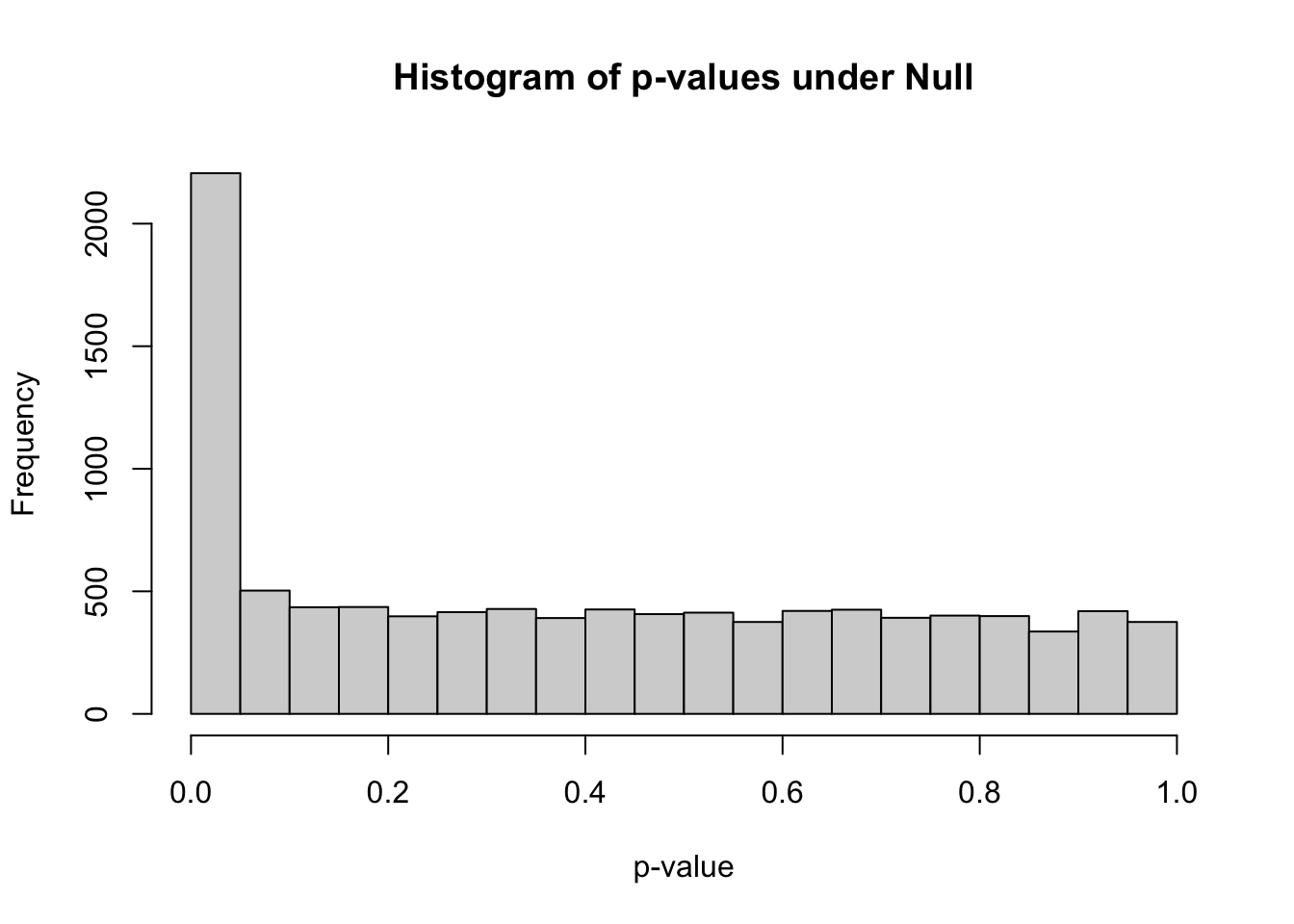
m_signif = sum(pvec_mix < 0.05) ## observed number of significant associations
m_expected = 0.05*nsim ## expected number of significant associations under the worst case scenario, where all features belong to the null
m_signif
## [1] 2206m_expected## [1] 500Under the null, we were expecting 500 significant columns by chance but got 2206
Q: how can we estimate the proportion of true positives?
We got 1706 extra columns, so it’s reasonable to expect that the extra significant results come from the alternative distribution (Yalt). So \[\frac{\text{observed number of significant} - \text{expected number of significant}}{\text{observed number of significant}}\] should be a good estimate of the true discovery rate. False discovery rate is defined as 1 - the true discovery rate.
thres = 0.05
FDR = sum((pvec_mix<thres & selectvec==0)) / sum(pvec_mix<thres)
## proportion of null columns that are significant among all significant
FDR
## [1] 0.1885766Note2
qqplots are great tools to compare distributions

QQplot Figure
## loading my qqunif function
devtools::source_gist("https://gist.github.com/hakyim/38431b74c6c0bf90c12f")
## Sourcing https://gist.githubusercontent.com/hakyim/38431b74c6c0bf90c12f/raw/fe087cf0519d4a3d71f0c8235f42cce4549438ac/qqunif.R## SHA-1 hash of file is 0b30870726d50889d1366a1f3b21942510a05128qqunif(pvec,main="null")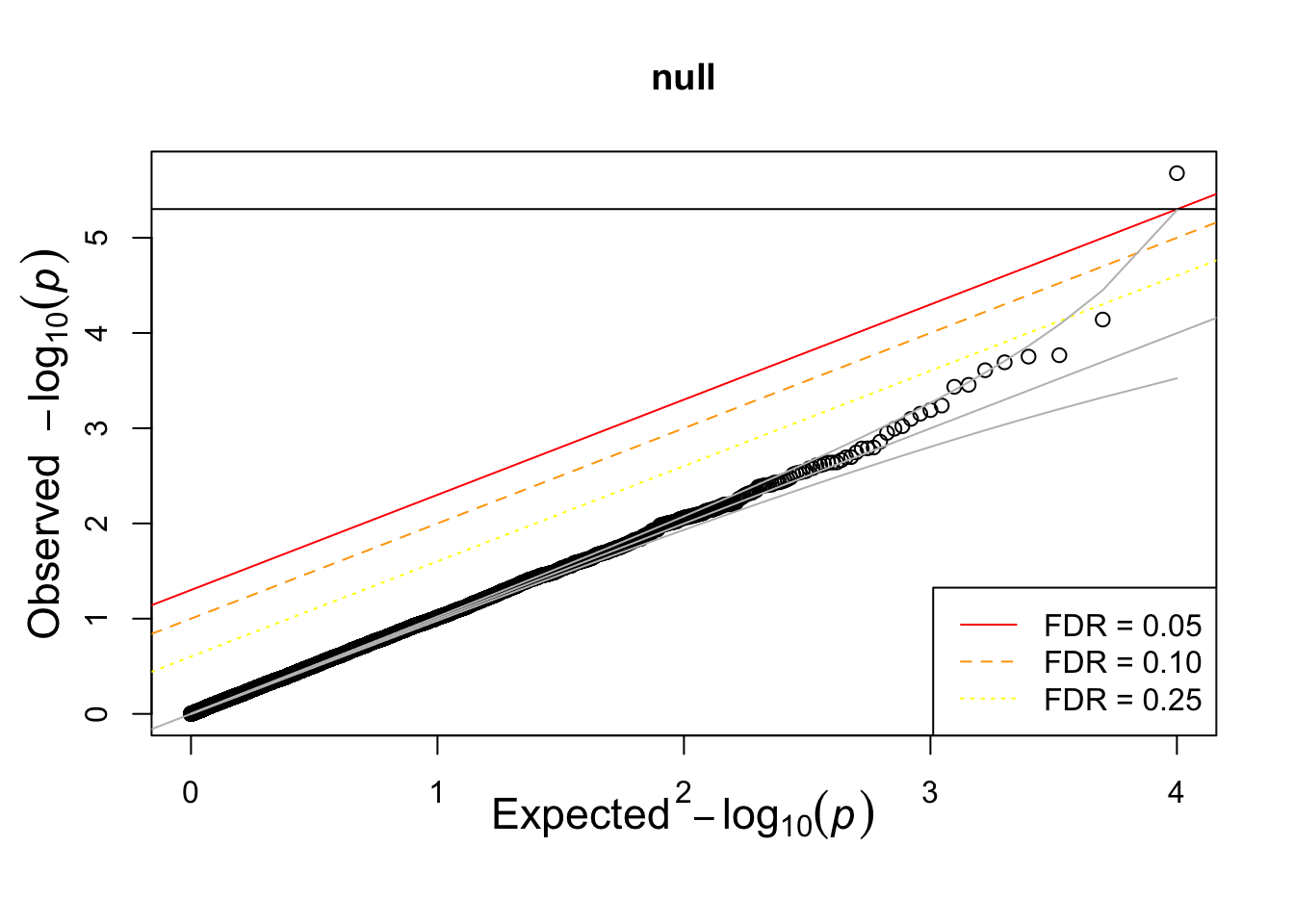
ind=order(pvec_mix,decreasing=FALSE)
qqunif(pvec_mix, col = selectvec[ind]*2 +1, main = 'mixture of null and alt')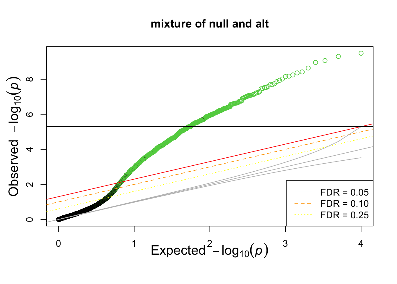
table(pvec_mix<0.05, selectvec)## selectvec
## 0 1
## FALSE 7580 214
## TRUE 416 1790count_table = t(table(pvec_mix>0.05, selectvec))
colnames(count_table) = c("Called significant", "Called not significant")
rownames(count_table) = c("Null true", "Alt true")
knitr::kable(count_table)| Called significant | Called not significant | |
|---|---|---|
| Null true | 416 | 7580 |
| Alt true | 1790 | 214 |
Common approaches to control type I errors
Assuming we are testing \(m\) hypothesis, let’s define the following terms for the different errors.
| Called Significant | Called not significant | Total | |
|---|---|---|---|
| Null true | \(F\) | \(m_0 - F\) | \(m_0\) |
| Alt true | \(T\) | \(m_1 - T\) | \(m_1\) |
| Total | \(S\) | \(m - S\) | \(m\) |
- Bonferroni correction assures that the FWER (Familywise error rate) \[P(F \ge 1|\text{Null})\] is below the acceptable type I error, typically 0.05. This can be too stringent and lead to miss real signals.
- pFDR (positive false discovery rate) \[E\left(\frac{F}{S} \rvert S>0\right)\]
- qvalue is the minimum false discovery rate attainable when the feature (SNP) is called significant
Next, we’ll calculate the qvalue.
We need a way to estimate \(m_0\)
 From Storey and Tibshirani PNAS
Use qvalue package to calculate FDR and
if (!requireNamespace("BiocManager", quietly = TRUE))
    install.packages("BiocManager")

BiocManager::install("qvalue")
Let’s check whether small qvalues correspond to true associations (i.e. the phenotype was generated under the alternative distribution)
qres = qvalue::qvalue(pvec)
qvec = qres$qvalue

qres_mix = qvalue::qvalue(pvec_mix)
qvec_mix = qres_mix$qvalue

plot(qvec_mix,col=selectvec*2 + 1, pch=selectvec + 1, lwd=selectvec*2 + 1) 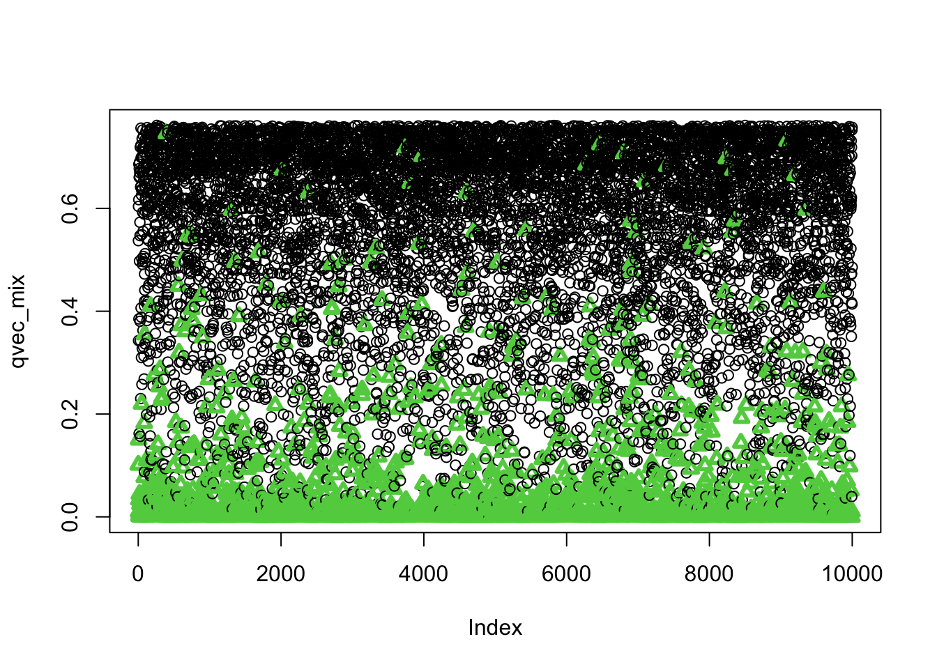
## using selectvec*2 + 1 as a quick way to get the vector to be 1 and 3 (1 is black 3 is green) instead of 1 and 2 (2 is read and can be difficult to read for color blind people)

ind=order(qvec_mix,decreasing=FALSE)
plot(sort(qvec_mix),col=selectvec[ind]*2 + 1, pch=selectvec[ind] + 1, lwd=selectvec[ind]*2 + 1) 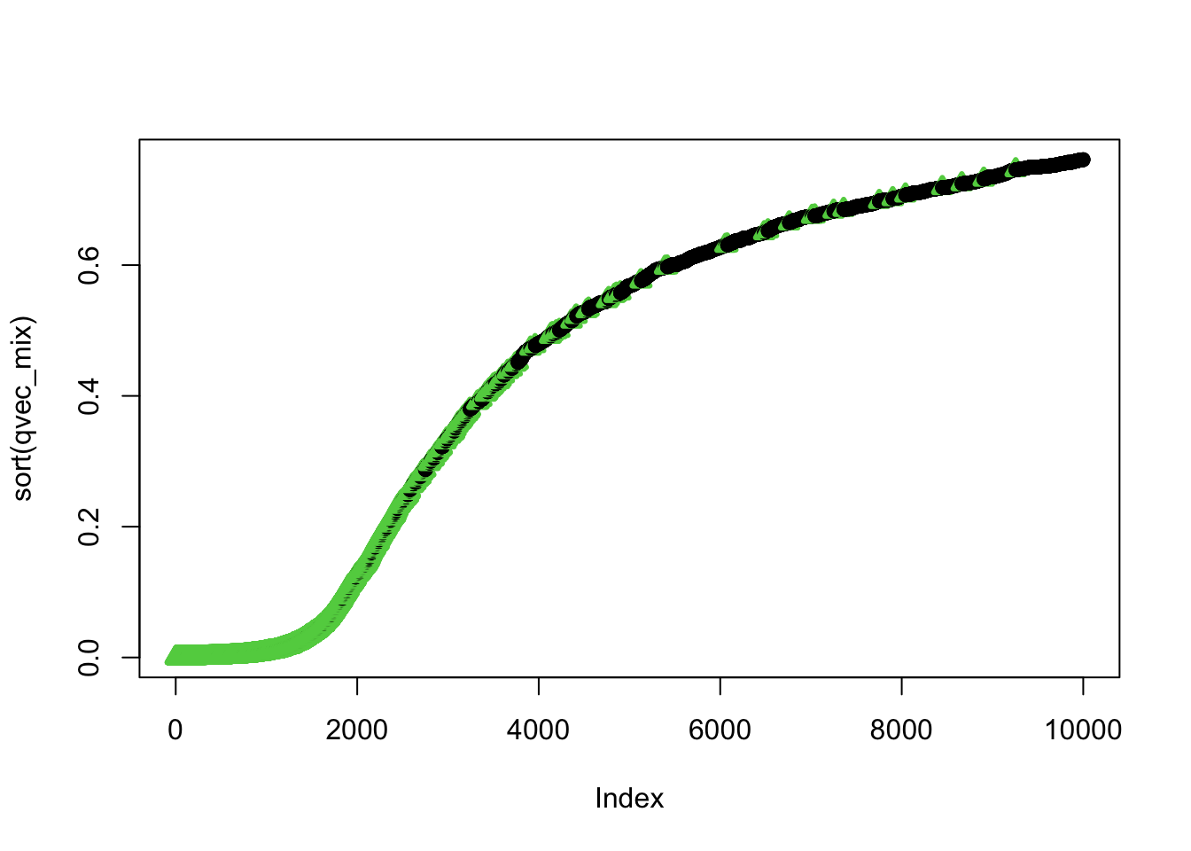
summary(qvec_mix) ## Min. 1st Qu. Median Mean 3rd Qu. Max.
## 0.0000019 0.2391430 0.5681539 0.4635186 0.6894836 0.7615203## distribution of qvlues and pvalues by causal status
boxplot(pvec_mix ~ selectvec, main='pvalue by causal status; 1=alt, 0=null')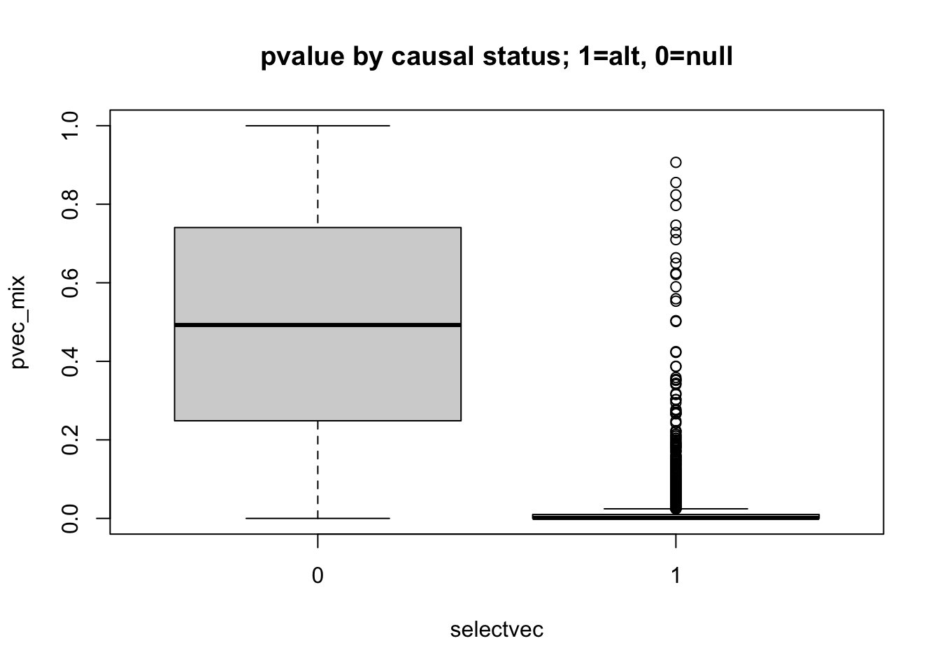
boxplot(qvec_mix ~ selectvec, main='qvalue by causal status; 1=alt, 0=null')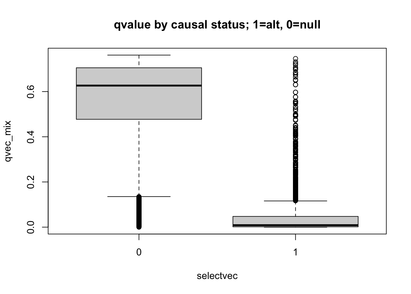
How do qvalues and pvalues relate to each other?
plot(pvec,qvec,main='qvalue vs pvalue for null')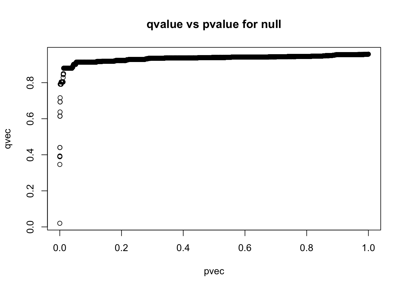
plot(pvec_mix,qvec_mix,main='qvalue vs pvalue for mixture of null and alt')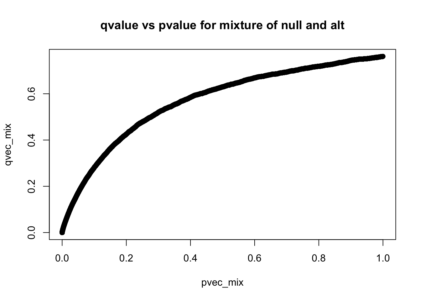
pi0 and pi1
pi0 is the proportion of null hypothesis which can be estimated using the qvalue package 1 - pi1 is the proportion of true positive associations. This is a useful parameter as we will see in later classes.
qres$pi0## [1] 0.9581828qres_mix$pi0## [1] 0.7616416References
Benjamini Y, Hochberg Y. Controlling the false discovery rate: a practical and powerful approach to multiple testing. Journal of the Royal Statistical Society B. 1995;57:289–300.
Storey JD, Tibshirani R. Statistical significance for genomewide studies. Proc Natl Acad Sci U S A. 2003;100(16):9440-9445. doi:10.1073/pnas.1530509100