Personal Genomes Project Data

Haky Im

2021-04-21

Goal

-[ ] download Personal Genome Project data (http://repgp.teamerlich.org/)

-[ ] analyze content, explore structure

-[ ] predict height and other phenotypes with PRS and compare to reported values

library(tidyverse)

## ── Attaching packages ─────────────────────────────────────── tidyverse 1.3.0 ──

## ✓ ggplot2 3.3.3     ✓ purrr   0.3.4
## ✓ tibble  3.1.0     ✓ dplyr   1.0.3
## ✓ tidyr   1.1.2     ✓ stringr 1.4.0
## ✓ readr   1.4.0     ✓ forcats 0.5.0

## ── Conflicts ────────────────────────────────────────── tidyverse_conflicts() ──
## x dplyr::filter() masks stats::filter()
## x dplyr::lag()    masks stats::lag()

library(RSQLite)
sqlite <- dbDriver("SQLite")
DATA="/Users/haekyungim/Box/LargeFiles/imlab-data/data-Github/web-data/2021-04-21-personal-genomes-project-data/"
WORK=DATA

Define environmental variables for convenience

DATA="/Users/haekyungim/Box/LargeFiles/imlab-data/data-Github/web-data/2021-04-21-personal-genomes-project-data/"
WORK=$DATA
PRSice=/Users/haekyungim/bin/PRSice_mac
BIN="/Users/haekyungim/bin"

## download sqqtl database with phenotypes?
cd $DATA
wget http://files.teamerlich.org/repgp/repgp-data.sqlite3 
wget http://files.teamerlich.org/repgp/repgp.vcf.gz

dbname <- paste0(DATA,"repgp-data.sqlite3") ## add full path if db file not in current directory
## connect to db
db = dbConnect(sqlite,dbname)
## list tables
dbListTables(db)

## [1] "ancestry_jkp"   "ancestry_pop"   "ancestry_supop" "users"

dbListFields(db, "users")

## [1] "id"       "sample"   "height"   "weight"   "human_id" "file_id"  "blood"   
## [8] "gender"   "race"

## convenience query function
query <- function(...) dbGetQuery(db, ...)

users = query("select * from users")
names(users)

## [1] "id"       "sample"   "height"   "weight"   "human_id" "file_id"  "blood"   
## [8] "gender"   "race"

users %>% count(race)

##                               race   n
## 1                                *  68
## 2 American Indian or Alaska Native   2
## 3                            Asian   6
## 4        Black or African American   1
## 5                Caucasian (White)   1
## 6               Hispanic or Latino   2
## 7                  Hispanic/Latino   3
## 8                            White 167

users  %>% count(gender)

##   gender   n
## 1      *  69
## 2 Female  46
## 3   Male 135

users %>% count(blood)

##   blood   n
## 1     * 111
## 2    A-  10
## 3    A+  41
## 4   AB-   1
## 5   AB+   4
## 6    B-   4
## 7    B+  16
## 8    O-  11
## 9    O+  52

users %>% ggplot(aes(height,fill=gender)) + geom_density(alpha=0.6) + ggtitle("Height by gender - Missing gender, *, has bi-modal distr.")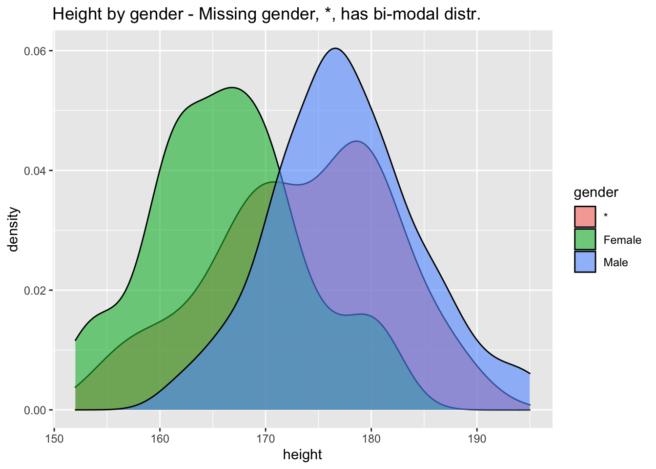

Download imputed genotype files

cd $DATA
for num in $(seq 22);
do
 wget http://files.teamerlich.org/repgp/repgp-imputed.chr${num}.vcf.gz
done

Create plink formatted genotype files. You will need plink2, which you can download from here

## install plink2 from https://www.cog-genomics.org/plink/2.0/
## more plink2 to ~/bin/
## ~/bin/plink2 --vcf repgp-imputed.chr22.vcf.gz    --make-bed --out repgp
cd $DATA
for num in $(seq 22);
do
~/bin/plink2 --vcf repgp-imputed.chr${num}.vcf.gz   --make-bed --out repgp.chr${num}
done

Choose a trait and download its GWAS summary statistics from this list https://uchicago.box.com/v/test-gtex-gwas-ukb-data

## here I chose sleep duration
cd $DATA
##wget https://uchicago.box.com/s/4gc4u1yr579qjbz8s6d27h8vb0h1yw1q
wget -O ukb_sleep_duration.gz https://uchicago.box.com/shared/static/4gc4u1yr579qjbz8s6d27h8vb0h1yw1q.gz
## height
wget -O ukb_height.gz https://uchicago.box.com/shared/static/2889tf5fx5d5ulll7otg4dltd1vogabh.gz

Create phenotype file

fam = read_tsv(glue::glue("{DATA}/repgp.fam"),col_names = FALSE)

## 
## ── Column specification ────────────────────────────────────────────────────────
## cols(
##   X1 = col_double(),
##   X2 = col_character(),
##   X3 = col_double(),
##   X4 = col_double(),
##   X5 = col_double(),
##   X6 = col_double()
## )

names(fam)[1:2] = c("FID","IID")
fam <- fam %>% select(FID, IID) %>% inner_join(users %>% select(sample,height,weight,gender), by=c("IID"="sample")) 
write_tsv(fam,file=glue::glue("{DATA}/phenodata.txt"))

## use --pheno-col to specify phenotype list
mkdir $WORK/output
Rscript $PRSice/PRSice.R --dir $PRSice \
    --prsice $PRSice/PRSice_mac \
    --base $WORK/ukb_height.gz \
    --target $WORK/repgp.chr# \
    --snp variant_id \
    --A1 effect_allele \
    --A2 non_effect_allele \
    --stat effect_size \
    --beta \
    --pvalue pvalue \
    --pheno-file $WORK/phenodata.txt \
    --pheno-col height \
    --bar-levels 5e-08,5e-07,5e-06,5e-05,5e-04,5e-03,5e-02,5e-01,1 \
    --fastscore \
    --binary-target F \
    --thread 2 \
    --out $WORK/output/height_score_all

Got the following error. Some SNP IDs are duplicated.

Error: A total of 14 duplicated SNP ID detected out of 
       6417846 input SNPs! Valid SNP ID (post --extract / 
       --exclude, non-duplicated SNPs) stored at 
       /Users/haekyungim/Box/LargeFiles/imlab-data/data-Github/web-data/2021-04-21-personal-genomes-project-data//output/height_score_all.valid. 
       You can avoid this error by using --extract 
       /Users/haekyungim/Box/LargeFiles/imlab-data/data-Github/web-data/2021-04-21-personal-genomes-project-data//output/height_score_all.valid

Try again including only the SNP list created by the previous run of PRSice, height_score_all.valid A1 is the effect allele in PRSice, similar to Plink’s default. Other software use different conventions so this sign is something that need to be checked carefully.

Rscript $PRSice/PRSice.R --dir $PRSice \
    --prsice $PRSice/PRSice_mac \
    --base $WORK/ukb_height.gz \
    --target $WORK/repgp.chr# \
    --snp variant_id \
    --A1 effect_allele \
    --A2 non_effect_allele \
    --stat effect_size \
    --beta \
    --pvalue pvalue \
    --pheno-file $WORK/phenodata.txt \
    --pheno-col height \
    --bar-levels 5e-08,5e-07,5e-06,5e-05,5e-04,5e-03,5e-02,5e-01,1 \
    --fastscore \
    --binary-target F \
    --thread 2 \
    --extract $WORK/output/height_score_all.valid \
    --out $WORK/output/height_score_all

This time it worked. This figure shows the correlation (squared) between prediction and actual values provided in the phenodata.txt file. In this dataset, using SNPs with p-values up to 0.005 yielded the most significant correlation. Next, we will plot the predicted and actual values to get a better sense of how well PRS is predicting.

Plot predicted vs actual height

## we already have the phenotype data in the fam variable
predicted_height = read_delim(glue::glue("{DATA}/output/height_score_all.best"),delim=" ")

## 
## ── Column specification ────────────────────────────────────────────────────────
## cols(
##   FID = col_double(),
##   IID = col_character(),
##   In_Regression = col_character(),
##   PRS = col_double()
## )

combined <- predicted_height %>% inner_join(fam,by=c("IID"="IID")) 

combined %>% ggplot(aes(PRS,height)) + geom_point()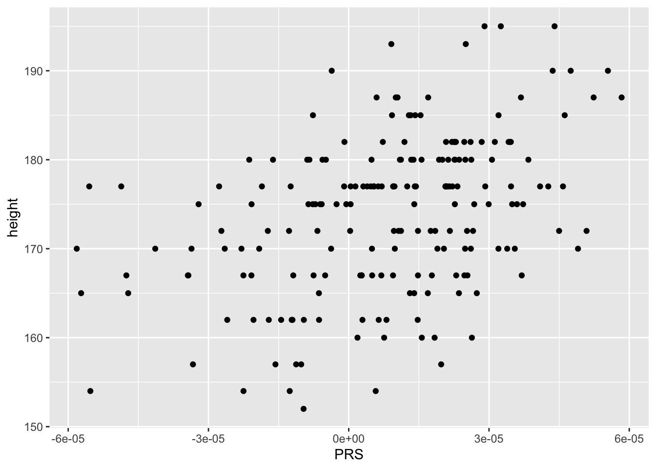

summary(lm(height ~ PRS,data=combined)) %>% coef()

##                Estimate   Std. Error    t value      Pr(>|t|)
## (Intercept)    172.6716 6.075067e-01 284.230021 1.916175e-259
## PRS         159197.1399 2.478220e+04   6.423849  9.758137e-10

Personal Genomes Project Data

Haky Im

2021-04-21

Reuse

Suggest changes

Citation