Goals and Introduction

In this lab we are going to use the PRSice software to take height GWAS results and predict height of the Personal Genome Project individuals using their genotype data.

Goals

• Download data from box
• Download PRSice
• Run exploratory analysis of data
• Run PRSice
• Plot observed versus predicted for height

Setup

library(tidyverse)

## ── Attaching packages ─────────────────────────────────────── tidyverse 1.3.1 ──

## ✓ ggplot2 3.3.5     ✓ purrr   0.3.4
## ✓ tibble  3.1.6     ✓ dplyr   1.0.8
## ✓ tidyr   1.2.0     ✓ stringr 1.4.0
## ✓ readr   2.1.2     ✓ forcats 0.5.1

## ── Conflicts ────────────────────────────────────────── tidyverse_conflicts() ──
## x dplyr::filter() masks stats::filter()
## x dplyr::lag()    masks stats::lag()

library(RSQLite)

sqlite <- dbDriver("SQLite")
DATA="/file/path/to/box/download"
WORK=DATA

wget https://github.com/choishingwan/PRSice/releases/download/2.3.3/PRSice_mac.zip

DATA="/file/path/to/box/download"
WORK=$DATA
PRSice=file/path/to/PRSice

cd $DATA

Exploration of the Data

dbname <- paste0(DATA,"repgp-data.sqlite3") ##This is just to create the file path to the sqlite3 file 
## connect to db
db = dbConnect(sqlite, dbname)
## list tables
dbListTables(db)

## [1] "ancestry_jkp"   "ancestry_pop"   "ancestry_supop" "users"

dbListFields(db,"users")

## [1] "id"       "sample"   "height"   "weight"   "human_id" "file_id"  "blood"   
## [8] "gender"   "race"

query <- function(...) dbGetQuery(db, ...)
users = query("select * from users")
names(users)

## [1] "id"       "sample"   "height"   "weight"   "human_id" "file_id"  "blood"   
## [8] "gender"   "race"

users %>% count(race)

##                               race   n
## 1                                *  68
## 2 American Indian or Alaska Native   2
## 3                            Asian   6
## 4        Black or African American   1
## 5                Caucasian (White)   1
## 6               Hispanic or Latino   2
## 7                  Hispanic/Latino   3
## 8                            White 167

users  %>% count(gender)

##   gender   n
## 1      *  69
## 2 Female  46
## 3   Male 135

users %>% count(blood)

##   blood   n
## 1     * 111
## 2    A-  10
## 3    A+  41
## 4   AB-   1
## 5   AB+   4
## 6    B-   4
## 7    B+  16
## 8    O-  11
## 9    O+  52

users %>% ggplot(aes(height,fill=gender)) + geom_density(alpha=0.6) + ggtitle("Height by gender - Missing gender, *, has bi-modal distr.")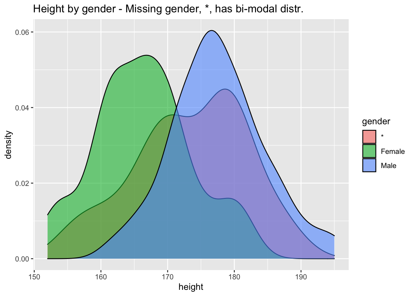

Running PRSice

fam = read_tsv(glue::glue("{DATA}/repgp.fam"),col_names = FALSE)

## Rows: 568 Columns: 6
## ── Column specification ────────────────────────────────────────────────────────
## Delimiter: "\t"
## chr (1): X2
## dbl (5): X1, X3, X4, X5, X6
## 
## ℹ Use `spec()` to retrieve the full column specification for this data.
## ℹ Specify the column types or set `show_col_types = FALSE` to quiet this message.

names(fam)[1:2] = c("FID","IID")
fam <- fam %>% select(FID, IID) %>% inner_join(users %>% select(sample,height,weight,gender), by=c("IID"="sample")) 
write_tsv(fam,file=glue::glue("{DATA}/phenodata.txt"))

mkdir $WORK/output

Rscript $PRSice/PRSice.R --dir $PRSice \
    --prsice $PRSice/PRSice_mac \
    --base $WORK/ukb_height.gz \
    --target $WORK/repgp.chr# \
    --snp variant_id \
    --A1 effect_allele \
    --A2 non_effect_allele \
    --stat effect_size \
    --beta \
    --pvalue pvalue \
    --pheno-file $WORK/phenodata.txt \
    --pheno-col height \
    --bar-levels 5e-08,5e-07,5e-06,5e-05,5e-04,5e-03,5e-02,5e-01,1 \
    --fastscore \
    --binary-target F \
    --thread 2 \
    --out $WORK/output/height_score_all

Plotting Observed Versus Predicted Height

## we already have the phenotype data in the fam variable
predicted_height = read_delim(glue::glue("{DATA}/output/height_score_all.best"),delim=" ")

## Rows: 568 Columns: 4
## ── Column specification ────────────────────────────────────────────────────────
## Delimiter: " "
## chr (2): IID, In_Regression
## dbl (2): FID, PRS
## 
## ℹ Use `spec()` to retrieve the full column specification for this data.
## ℹ Specify the column types or set `show_col_types = FALSE` to quiet this message.

combined <- predicted_height %>% inner_join(fam,by=c("IID"="IID")) 

combined %>% ggplot(aes(PRS,height)) + geom_point()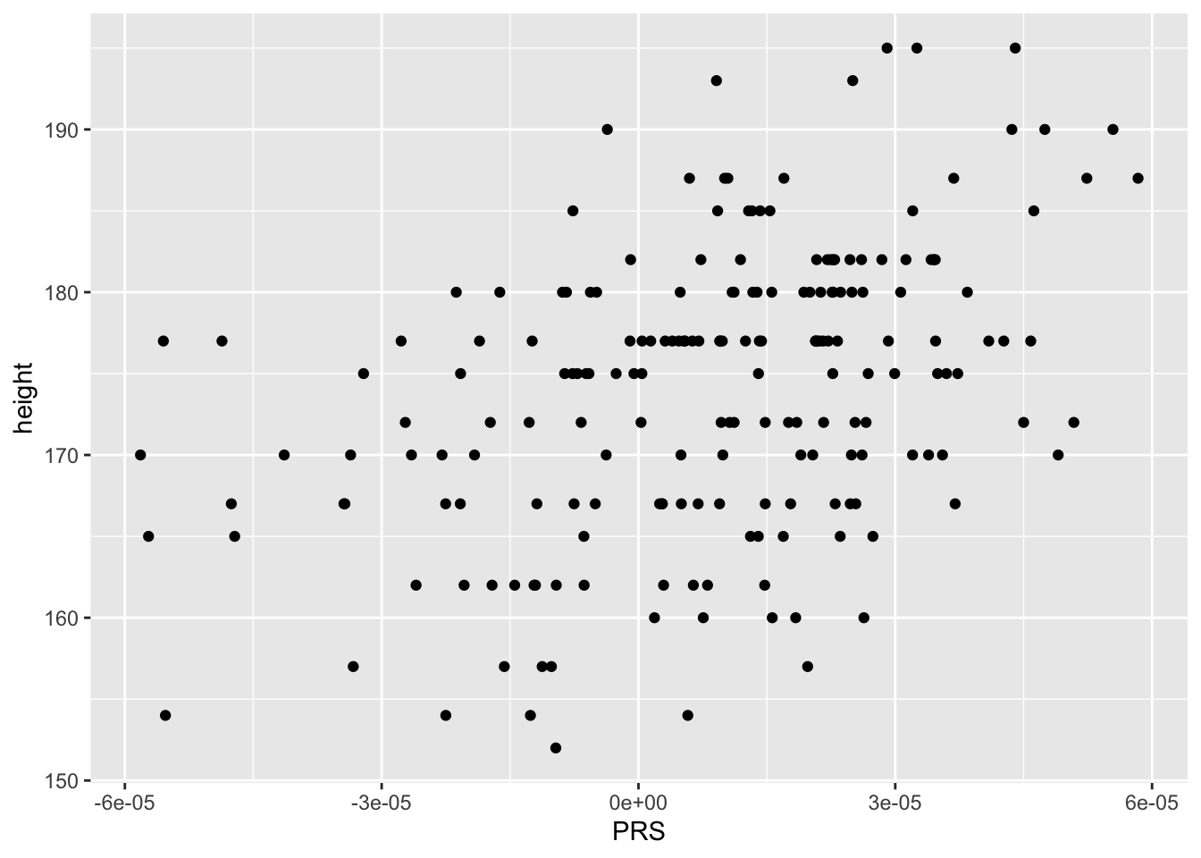

summary(lm(height ~ PRS,data=combined)) %>% coef() 

##                Estimate   Std. Error    t value      Pr(>|t|)
## (Intercept)    172.6716 6.075067e-01 284.230021 1.916175e-259
## PRS         159197.1399 2.478220e+04   6.423849  9.758137e-10