Lecture 6

Haky Im

2021-04-13

Categories: Lecture

Learning Objectives

Explain various methods to control for population structure
Use mixed effects model approach to correct for population structure
Use LD Score regression to distinguish between population structure and polygenicity driven inflation

Notes

Find the class notes here

Review connection between Zscore, p-value, Chi2 statistic

Notice that, under the null hypothesis, the estimated effect size divided by the standard error behaves like a normal(0,1) random variable when the sample size is large enough:

\[ Z = \frac{\hat\beta}{\text{se}(\hat\beta)}\] \[Z \approx N(0,1) ~~~~~~ \text{as } n \rightarrow \infty\] Let’s simulate zscore vector under the null hypothesis.

nsim = 5000
set.seed(2021021001)
zvec = rnorm(5000, mean=0, sd=1)

Calculate the p-value (probability that a normal r.v. will be as large or larger in magnitude than the observed |zscore|

pvec = pnorm(-abs(zvec)) * 2 ## two-tailed
## check pvec is uniformly distributed
hist(pvec,main="is this uniformly distributed?")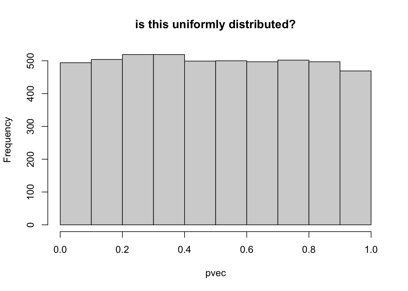

remember that if square the a normal r.v. you get chi2 r.v. with one degree of freedom

z2vec = zvec^2
## compare with chi2 rv. with 1 degree of freedom by simulating chi2,1 and qqplot
chi2vec = rchisq(nsim,df=1)
qqplot(chi2vec,z2vec,main="compare of zscore^2 and a chi2 r.v."); abline(0,1)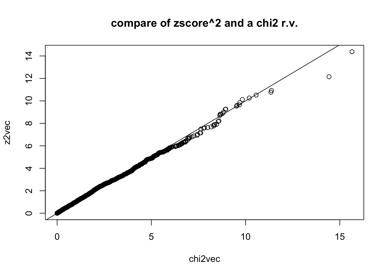

## for reference, let's compare two chi2,1 r.v.'s qqplot
chi2vec_2 = rchisq(nsim,df=1)
qqplot(chi2vec,chi2vec_2,main="qqplot of two chi2,1 r.v."); abline(0,1)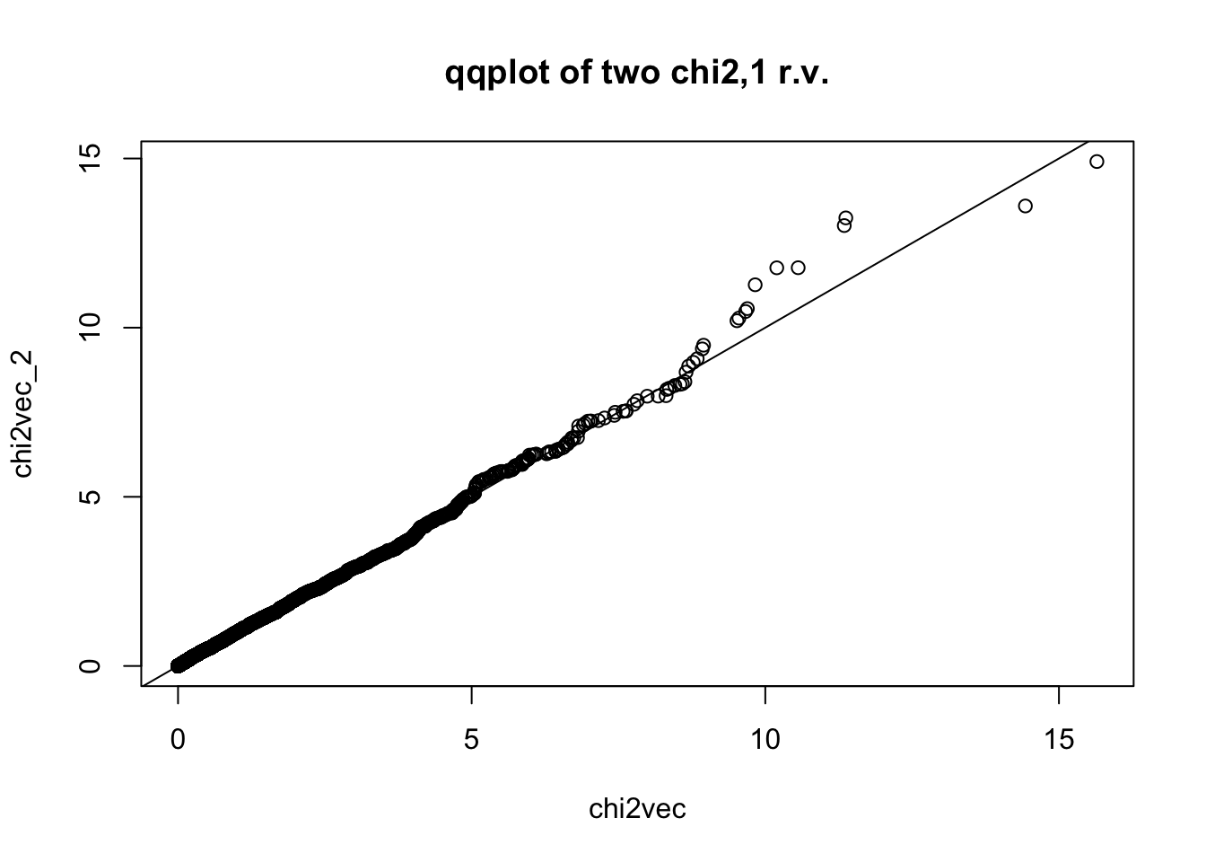

Sometimes you get the p-value instead of the zscore, you can generate chi2 by inverting the relationship.

chi2vec_from_p = qnorm(pvec / 2)^2
qqplot(chi2vec,chi2vec_from_p,main="chi2 from pvalue vs chi2 r.v."); abline(0,1)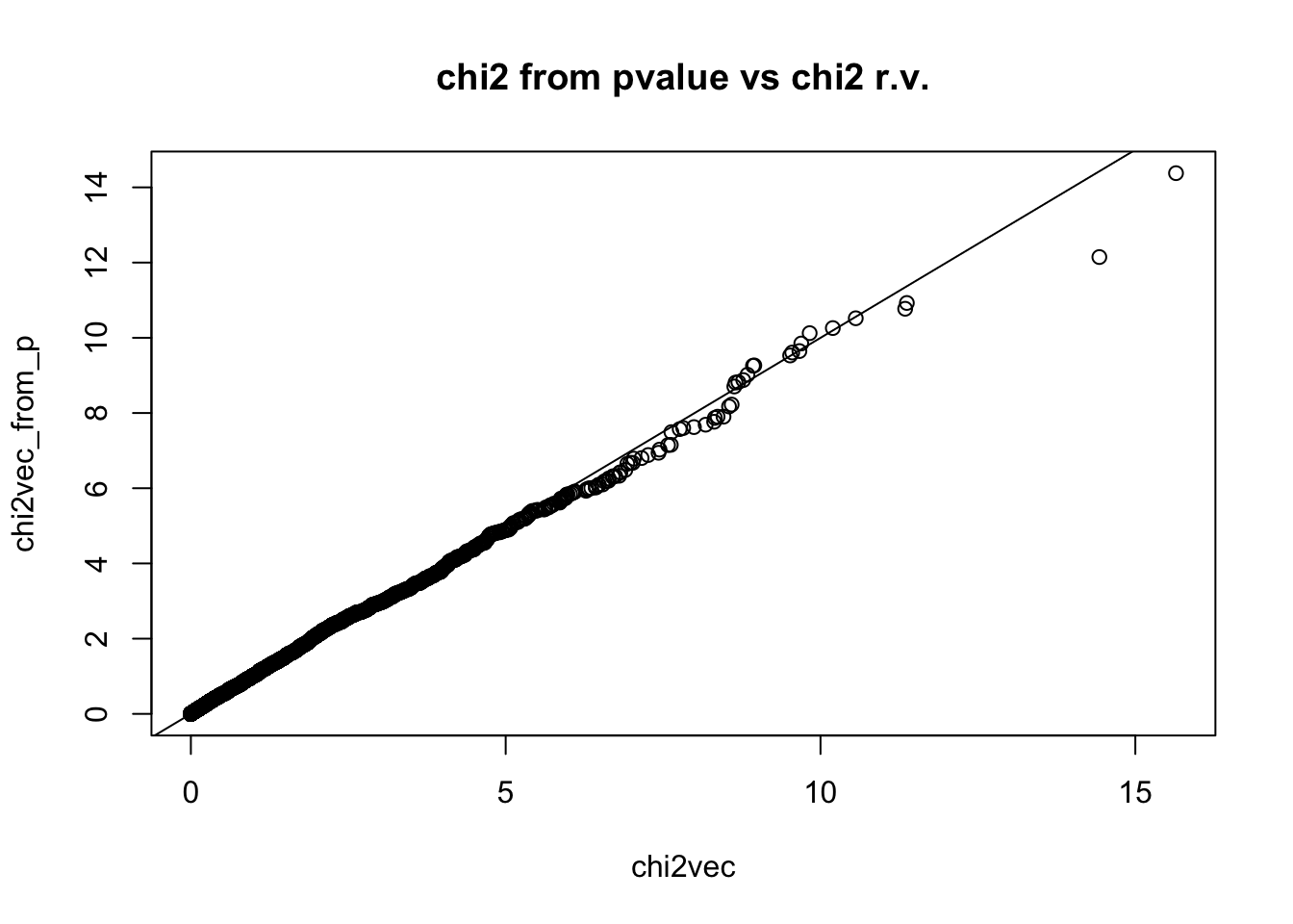

Homework problem

Write an R function to calculate the chi2 statistics as a function of the estimated effect size, \(\hat\beta\), and the standard error of the estimated effect size, se(\(\hat\beta\)).

References

B. Devlin and Kathryn Roeder (1999) “Genomic Control for Association Studies”, Biometrics, Vol. 55, No. 4, 997-1004.
H. M. Kang, J. H. Sul, S. K. Service, N. A. Zaitlen, S.-Y. Kong, N. B. Freimer, C. Sabatti, and E. Eskin, “Variance component model to account for sample structure in genome-wide association studies,” Mar. 2010.
A. L. Price, N. A. Zaitlen, D. Reich, and N. Patterson, “New approaches to population stratification in genome-wide association studies,” Nat Rev Genet, vol. 11, no. 7, pp. 459–463, Jun. 2010. B. K. Bulik-Sullivan, P.-R. Loh, H. K. Finucane, S. Ripke, J. Yang, N. Patterson, M. J. Daly, A. L. Price, and B. M. Neale, “LD Score regression distinguishes confounding from polygenicity in genome-wide association studies,” Nat Genet, vol. 47, no. 3, pp. 291–295, Feb. 2015.